Using GNSS Phase Reflectometry on Maui’s Haleakalā

Read Richard Langley’s introduction to this article: “Innovation Insights: Science in paradise”

Originally developed for navigation and timing applications, signals from global navigation satellite systems (GNSS) are now commonly used for geophysical remote sensing applications, including observation of Earth’s surface and atmosphere using near sea-level ground stations as well as mountaintop, airborne and spaceborne platforms. GNSS reflectometry (abbreviated GNSS-R), which is the technique of using reflected signals to measure properties of Earth’s surface, has been a growing area of research and application for GNSS remote sensing. Notably, the Cyclone Global Navigation Satellite System (CYGNSS) satellite mission produces delay-Doppler maps (DDMs) that are used to monitor ocean surface wind speeds during hurricanes. Meanwhile, terrestrial and airborne GNSS-R has been used to monitor soil moisture, snow depth and vegetation growth. One area of increasing interest is precision reflectometry using signal carrier-phase measurements. The first attempt to perform precision (phase) altimetry over sea ice using GPS reflectometry measurements from the low-Earth orbiting TechDemoSat-1 was reported by researchers in 2017. Subsequently, researchers demonstrated the use of reflections collected by a Spire satellite to perform altimetry over Hudson Bay and the Java Sea and how reflections off ice in the polar regions can be used to measure ionospheric total electron content over the polar caps. While these demonstrations of GNSS-R for precision carrier-phase-based reflectometry are promising, more work needs to be done to characterize when carrier-based altimetry is feasible and what challenges it faces.

To study the challenges associated with processing reflected and low-elevation-angle radio occultation signals, the University of Colorado (CU) Boulder Satellite Navigation and Sensing (SeNSe) Laboratory has deployed a GNSS data collection site on top of Mount Haleakalā on the island of Maui, Hawaii. Recent collection campaigns aim to use this site as a testbed for GNSS-R algorithms that utilize multi-frequency and multi-polarization measurements. Previously, we carried out delay map processing for left-hand circular (LHC) and right-hand circular (RHC) polarizations for L1 and L2 GPS signals. Those results validate the open-loop processing methodology and provide an initial assessment of the data quality. We observed that the received reflected signals show deep and rapid fading in amplitude. In the work reported in this article, we extend our assessment to triple-frequency GPS (L1CA, L2C, L5Q) signals and document our methodology for extraction of the signal carrier phase. Our initial results indicate that coherent signal phase extraction is challenging, and may not be feasible for this particular experiment setup. We discuss ways in which the experiment may be improved for the purpose of obtaining coherent ocean surface reflections in the future.

EXPERIMENT BACKGROUND

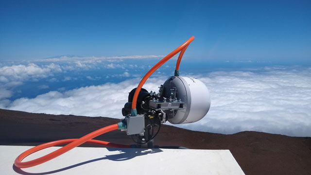
The current form of the CU SeNSe Lab Mount Haleakalā GNSS experiment was deployed in June 2020. It consists of a side-facing dual-polarization horn antenna, which is shown in the left panel of FIGURE 1, along with a zenith-facing reference antenna. The horizontally- and vertically-polarized wideband signals from the horn antenna are fed into front-end hardware and are combined using 90-degree phase combiners to form LHC and RHC polarized signals, which are then recorded by a set of Ettus Universal Software Radio Peripherals (USRPs). Meanwhile, the signal from the reference antenna is sent to a Septentrio PolaRxS receiver. The right panel in Figure 1 illustrates the system setup. Note that the Septentrio onboard oven-controlled crystal oscillator is used to drive the USRPs. This allows us to use the Septentrio outputs to estimate the receiver clock variations and use them in the receiver clock component of our open-loop models, which we discuss below.

Figure 1: The side-facing horn antenna in its radome enclosure (left panel) and the hardware block diagram of the data collection system (right panel). (All figures provided by the authors)

Each USRP can record up to four signals at two different mixdown frequencies, allowing for recording of both the RHC and LHC polarized signals on up to four different bands. The first USRP records the L1 and L2 bands with center frequencies at 1575.42 and 1227.6 MHz, respectively, at a bandwidth of 5 MHz. The second USRP records the L5 and E6/B3 bands at center frequencies of 1176.45 and 1271.25 MHz and at a 20 MHz bandwidth. TABLE 1 lists the IDs for each receive channel along with its corresponding band, polarization and sampling rate. Note that the recorded signals covering the E6 band also capture BeiDou B3 signals, but we restrict our analysis to GPS L1, L2 and L5 signals in this article. The samples from these USRPs are written to disk along with the Septentrio Binary Format (SBF) output of the PolaRxS receiver.

Table 1: Receiver IDs with corresponding band and polarization.

Starting in June 2021, periodic collections were taken for around one hour at a time, which is about the amount of time it takes for a GPS satellite to pass from an elevation angle of 0 degrees to one of more than 20 degrees. The collection times were adjusted to target the passes of satellites whose specular reflection point passed within the azimuthal range of the horn antenna, which faces roughly to the south and has a beam width of around 60 degrees. FIGURE 2 summarizes the available datasets from the first month of collections. The right-most panels of FIGURE 3 show examples of the specular track for GPS PRN 6 as it sets over the horizon on June 13, 2022, at around 12:00-13:00 UT. This is the pass on which we focus in this work, since PRN 6 transmits the L1CA, L2C and L5 signals and consistently had a specular point in our region of interest.

Figure 2: Available data during the first month of collections. The average significant wave height in the region south of Haleakalā is also plotted. Numbers near the bottom indicate the datasets analyzed for this article.

METHODOLOGY

Our processing method for open-loop tracking of the reflected GNSS signals is based on our previous work in which we produced DDMs and delay maps of the signal-to-noise ratio (SNR) measurements for multiple signal frequencies and received polarizations.

Pseudorange Model. We start by generating a model of the pseudorange for both the direct and reflected signal. The model only needs to be accurate down to the chip level, since we correlate across several chips of delay for the received signals. Setting a somewhat arbitrary accuracy requirement of 0.5 chips (equivalent to a delay of around 150 meters for L1CA/L2C or 15 meters for L5 signals), allows us to ignore path delays from the ionosphere and troposphere, which should only account for up to several meters of delay. The model has three terms that we estimate relative to GPS System Time (GPST): the receiver clock error, the satellite transmitter clock error and the geometric range. We use a surveyed position of the horn antenna along with International GNSS Service precise orbit and clock products for the transmitter clock error and positions. These allow us to compute the transmitter clock error and path delay for the direct signal. The reflected signal path delay can be found by computing the specular reflection point on the WGS84 ellipsoid and adding the distances from the transmitter to the specular point and the specular point to the receiver. The remaining term to estimate is the receiver clock error. Recall that our USRPs are driven by the Septentrio internal oscillator. Therefore, the clock error in Septentrio measurements is associated with variations in the reference oscillator for the USRPs. We utilize a geodetic detrending technique to estimate these clock variations and apply them to our pseudorange model. To construct the full receiver clock error, we estimate the time-alignment of the samples near the beginning of the collections to GPST by tracking one minute of a strong, mid-elevation-angle satellite and decoding its timing information. This provides us with an estimate of GPST at the start of the file, which we can use to construct a full estimate of the GPST at any sample in the file. Also, given our pseudorange model, we can find the received code phase and the Doppler frequency.

Figure 3: Example of delay maps from GPS PRN 6. The panels to the left show delay maps for the L1CA, L2C and L5 signals, both RHC and LHC polarizations. The bottom panel shows the corresponding elevation angle over the duration of the pass. The maps to the right show the specular point location during the pass, along with a contour of the WW3 model for significant wave height and swell-significant wave height.

Signal Correlation. Using the established code phase and Doppler models, we generate correlations for both reflected and direct signals. We correlate a reference signal over each 1-millisecond interval, and for sanity-checking purposes, we compute correlations over ± 3 chips at 0.5 chip spacing. This results in in-phase and quadrature (I/Q) correlation outputs every 1 millisecond. The left panels in Figure 3 show examples of the processed reflected signals for RHC and LHC polarization L1CA, L2C and L5Q signals from PRN 6 on June 13, 2021, at 12:00-13:00 UT. Note that as the satellite sets, at around 4 degrees elevation angle, the reflected signals merge with the stronger direct signal on the L1 and L2 signals. This happens later on L5 due to its higher bandwidth. We use the 0.0 chip bin to obtain I/Q outputs for carrier-phase processing for L1 and L2. For L5, we use the 0.0, -0.5, or -1.0 chip bin to account for model mismatch toward the end of the file.

Signal Fading and the WW3 Ocean Model. An eventual goal of the Haleakalā reflectometry experiment is to compare the characteristics of processed reflected signals with the ocean surface parameters near the specular point and glistening zone. To this end, we have incorporated data from the Hawaii regional WaveWatcher 3 (WW3) model. The model outputs information about wave height, direction and period due to both wind and swell, and has a resolution of around 5 kilometers. The data from this model is available in NetCDF format from several web services. The right panels of Figure 3 show contours of the wind- and swell-significant wave height in the South Haleakalā region. Meanwhile, note that the reflected signals (left panels) show high variability in the received power throughout the duration of the collection. While we hoped to be able to immediately observe a correlation between these wave parameters and the power fluctuations, it is clear that we need additional processing to tease out such a signal, and the changing satellite geometry will likely make this difficult to observe and validate. Even still, our results at the end of this article will show that there is likely some correlation between fading and wind parameters, though to what extent is unknown. Finally, note that the LHC polarizations (RX6, RX8, RX2) show much stronger reflected signals than the RHC polarizations. Since we are interested in processing the phase for the reflected signals, we report exclusively on the use of the LHC polarization signals in the rest of this article.

Carrier-Phase Processing. Once the correlations are performed, we take the I/Q correlations for both direct and reflected signals and process them to retrieve the cleaned reflected signal phase. The first series of steps in this process involve processing the direct signal to determine navigation / overlay symbol alignment and to estimate any residual phase fluctuations, which are mostly due to unmodeled receiver clock fluctuations. FIGURE 4 illustrates this process for the L1CA signal. The raw I/Q correlations are shown in the top panel. To these we apply a Costas phase-lock loop (PLL) to track the residual phase fluctuations without being sensitive to navigation / overlay symbol transitions. Next, we remove these residual phase fluctuations to obtain the detrended I/Q values.

Figure 4: The I/Q data cleaning process for the L1CA direct signal.

As shown in the second panel, these quadrature components of the detrended I/Q values are centered at zero while the in-phase component now shows the data bits / overlay symbols. We use the detrended I/Q values to estimate the navigation bit sequence on the L1CA and L2C signals. Likewise, we estimate the alignment of the Neumann-Hoffmann overlay sequence for the L5 signal. Finally, we wipe off the estimated data bits or overlay sequence to verify the procedure. The results of wiping off the estimated navigation bits for the L1CA signal are shown in the third panel of Figure 4.

Having obtained the residual phase fluctuations and navigation / overlay symbols for the direct signal, we next apply these to clean up the reflected signal. Specifically, we remove residual phase fluctuations from the raw reflected signal I/Q values and then wipe off the corresponding navigation bits or overlay code. FIGURE 5 shows an example of the reflected I/Q data before and after this procedure. The navigation bits are clearly removed, but the reflected signal still shows fairly significant fluctuations in the cleaned I/Q values. It is from these values that we hope to extract the residual reflected signal phase.

Figure 5: The reflected signal raw I/Q (top) and the I/Q after detrending and wiping off navigation bits for the L1CA signal.

Under coherent conditions, the phase of the clean reflected I/Q data should contain only the unmodeled effects, including any signature of ocean surface height variation. However, the effect of multipath due to the rough ocean surface causes fluctuations in the received signal amplitude and phase, and can additionally cause cycle slips when we unwrap the phase. To filter out these cycle slips, we apply our simultaneous cycle slip and noise filtering (SCANF) method, which is essentially just a Kalman filter PLL with an additional step that tries to estimate and remove cycle slips. The figures in the next section show the results of applying this entire procedure to the reflected signals. The black and blue lines show the phase before and after applying SCANF. The reflected signal I/Q SNR is also included for reference. Note how the jumps in the black line coincide with SNR fades, and the blue line effectively recreates the phase trend of the black line without these jumps. This is good qualitative evidence that the SCANF algorithm was effective.

RESULTS

FIGURES 6, 7, 8, 9, 10, and 11 show the reflected signal SNR and phase for GPS PRN 6 on 6 different days. Note that these days correspond to the marked days in Figure 2, from which we observe that the wind-significant wave height is relatively high on days 1, 5, and 6, moderate on days 2 and 3, and relatively low on day 4. We noticed that the SNR fluctuations on days 1, 5, and 6 are comparatively more frequent than on other days, which we believe may be a signature of the ocean surface conditions. A more detailed analysis of this result is a topic for our future work.

Figure 6: Reflected signal residual phase before (blue) and after (black) applying the SCANF filtering for the June 11, 2021 dataset. Amplitude and phase are shown in alternating panels for L1CA, L2C and L5 respectively.

Figure 7: Phase processing results for June 13, 2021.

Overall, we observe that the phase trend is not consistent across the three signals (L1CA, L2C, L5) for any of the days. With all the multipath signatures in the cleaned reflected signal, it was uncertain whether the extracted phase will be useful for applications such as ocean surface altimetry, and these qualitative results suggest that they probably will not be. However, season and hours of the day that were processed for our work discussed in this article are very limited. It is possible that processing more data will shed further insight onto whether the reflected signal phase is usable in this experiment.

Figure 8 Phase processing results for June 21, 2021.

Figure 9: Phase processing results for June 25, 2021.

ACKNOWLEDGMENTS

The Haleakalā data collection system has been established with support from the University of Hawaii Institute of Astronomy, and the Air Force Research Laboratory. The authors appreciate the assistance from Michael Maberry, Rob Ratkowski, Daniel O’Gara, Craig Foreman, Frank van Graas and Neeraj Pujara. This research is funded by a subaward from the National Oceanic and Atmospheric Administration through the University Corporation for Atmospheric Research to CU Boulder and with partial funding support from the NASA Commercial Smallsat Data Acquisition program.

This article is based on the paper “Initial Carrier Phase Processing for the Haleakala Mountaintop GNSS-R Experiment” presented at ION ITM 2023, the 2023 International Technical Meeting of the Institute of Navigation, Long Beach, California, Jan. 23–26, 2023.

Figure 10: Phase processing results for July 1, 2021.

Figure 11: Phase processing results for July 5, 2021.

BRIAN BREITSCH is a postdoctoral fellow at the University of Colorado (CU) Boulder, where he received his Ph.D. in aerospace engineering sciences.
JADE MORTON is a professor in the Ann and H.J. Smead Department of Aerospace Engineering Sciences and the director of the Colorado Center for Astrodynamics Research at CU Boulder.