No audio available for this content.

nonregistered, of georeferenced images from four UAV flights.
By Christian Eling, Lasse Klingbeil, Markus Wieland, Erik Heinz and Heiner Kuhlmann
Direct georeferencing with onboard sensors is less time-consuming for data processing than indirect georeferencing using ground control points, and can supply real-time navigation capability to a UAV. This is very useful for surveying, precision farming or infrastructure inspection. An onboard system for position and attitude determination of lightweight UAVs weighs 240 grams and produces position accuracies better than 5 centimeters and attitude accuracies better than 1 degree.
Data acquisition from mobile platforms has become established in many applications recently, particularly using unmanned aerial systems (UASs). Unlike other mobile platforms, unmanned aerial vehicles (UAVs) can overfly inaccessible and also dangerous areas. Furthermore, they can get very close to objects to collect high-resolution data with low-resolution sensors, and they enable approach from all viewing directions without physical contact. UAVs now see use in precision farming for phenotyping or plant monitoring, and in infrastructure inspection and surveying.
Data acquisition from mobile platforms has become established in many applications recently, particularly using unmanned aerial systems (UASs). Unlike other mobile platforms, unmanned aerial vehicles (UAVs) can overfly inaccessible and also dangerous areas. Furthermore, they can get very close to objects to collect high-resolution data with low-resolution sensors, and they enable approach from all viewing directions without physical contact. UAVs now see use in precision farming for phenotyping or plant monitoring, and in infrastructure inspection and surveying.
This article addresses lightweight UAV use for mobile mapping and uses the term micro aerial vehicle (MAV) throughout. MAVs can generally be characterized as having a weight limit of 5 kilograms and a size limit of 1.5 meters.
We focus on the development of a real-time capable, direct georeferencing system for MAVs, since spatial and time restrictions often exclude the possibility of deploying ground control points for an indirect georeferencing. The demand for the real-time capability results from the aim to also use the georeferencing for autonomous navigation of the MAV and to enable a precise time synchronization of the onboard sensors. Furthermore, a real-time direct georeferencing also offers the opportunity to process collected mapping data during flight.
Mapping on demand. The goal of this research project, funded by the Deutsche Forschungsgemeinschaft (DFG), is to develop an MAV that can identify and measure inaccessible three-dimensional objects by use of visual information. A major challenge within this project comes with the term “on demand.” This means that apart from the classical mapping part, where 3D information is extracted from aerial images, the MAV is intended to fly fully autonomously on the basis of a high-level user inquiry. During the flight, obstacles must be detected and avoided. To extract semantic information that can be used to refine the trajectory planning, the mapping data has to be processed in real time. When the georeferencing information is used as initial values for the bundle adjustment, the image processing can be significantly accelerated.
Figure 1 shows the current MAV platform developed in this project. We customized an MAV kit to a coaxial rotor configuration, replaced the centerplates with more stable carbon-fibre plates to stabilize the system, and installed the direct georeferencing and the mapping sensors. The two stereo camera pairs, pointing forward and backward, act as an additional sensory input for the position and attitude determination; the 5M-pixel industrial camera with global shutter is the actual mapping sensor. The PC board is used for onboard image processing, flight planning and machine control; the Wi-Fi module enables a connection to a ground station.

Although the direct georeferencing system must be small and lightweight, accuracy requirements for its position and attitude determination are high. Generally, these accuracy requirements are different for the machine control, navigation and mapping purposes.
In our project, the MAV is intended to maintain a safety distance of about 0.5 meter to obstacles. Hence, a position accuracy of 0.1 meter is sufficient for the navigation. The absolute attitude accuracy should be in the range of 1 to 5 degrees. For machine control, relative information is more important, and for this the accuracies should be slightly higher.
For mapping purposes, the positions and attitudes have to be known better, since the absolute georeference of the final product (for example, a high-resolution 3D model of a building) is based on the positions and attitudes from the direct georeferencing system. Therefore, the position accuracy should be in the range of 1–3 cm and the attitude accuracy should be better than 1 degree. The relative accuracy of the exterior camera orientation can be improved by a photogrammetric bundle adjustment, but systematic georeferencing errors should be avoided.
To summarize:
- The weight of the system has to be less than 500 grams (g), to be applicable on MAVs.
- Especially for the control and navigation, the system has to be real-time capable.
- All sensors have to be synchronized and outages of single sensors should be bridgeable by other sensors.
- The system is intended to provide accurate positions (σpos < 5 cm) and attitudes (σatt < 1 deg) during flights.
- The integration of data from additional sensors, such as cameras, should be possible.
The ability to include additional sensors to the system was, apart from the size and the weight constraint, the main reason for developing a proprietary system instead of using a commercial unit with similar capabilities.
Direct Georefencing
The current version of the system weighs 240 g without GPS antennas (see figure 2). To reduce weight, the antennas were dismantled, reducing their weight from 350 g to 100 g. However, since the antenna reference point got lost in this process, the antennas had to be recalibrated in an anechoic chamber for further use. By comparison to the original antennas, the dismantling led to significant changes in the phase center offsets (circa 4 cm in the Up, < 1 mm in the North and East component) and in the phase center variations (< 5 mm) of the antennas.

Figure 3 shows a flow chart of the direct georeferencing system with the sensors and the main calculation steps. The system consists of a dual-frequency GPS receiver, a single-frequency GPS receiver, an inertial measurement unit (IMU) and a magnetometer. The dual-frequency receiver is the main positioning device. Together with the GPS raw data from the master station (carrier phases ϕM, pseudoranges PM), which is transmitted via a radio module, the data of the dual-frequency receiver (ϕR, PR) is used for an RTK positioning, leading to centimeter position accuracies.

In collaboration with the data of the single-frequency receiver (ϕB, PB), the data of the dual-frequency receiver is also used for GPS attitude determination. The corresponding GPS antennas of these two receivers form a short baseline (baseline length = 92 cm) on the MAV. The determination of the baseline vector in an e-frame (Earth-fixed) enables yaw and the pitch-angle determination.
The tactical-grade micro-electro-mechanical (MEMS) IMU, which includes three-axes gyroscopes, accelerometers and magnetometers, provides angular rates (ω), accelerations (a) and magnetic field observations (h) with high rates (100 Hz) for position and attitude determination. To be unaffected by the electric currents as much as possible, an additional magnetometer is placed on the outer end of one of the rotor-free MAV arms.
The direct georeferencing system further consists of a processing unit, which is a reconfigurable IO board, including a field programmable gate array (FPGA) and a 400-MHz processor. In this combination, the FPGA is used for fast parallel communication with the sensors. Afterwards, the preprocessed sensor data are provided to the 400-MHz processor via direct memory accesses, avoiding delays and supporting the system’s real-time capabilities. Finally, the actual position and attitude determination is carried out on the 400-MHz processor.
Methodologies
All position and attitude determination algorithms running on the system were developed in-house. Generally, the integration of these steps could be realized in one tightly coupled approach. Nevertheless, in the current implementation, we decided to separate the different raw data calculation steps, and we only use interactions at the level of parameters. This approach has the advantage that the integration is more reliable and more practical in the real-time programming.
GPS/IMU integration. In this calculation step, all available sensory input is fused to determine the best position and attitude of the system that is currently available. The GPS and the IMU measurements complement each other well, since the IMU provides short-term stable high-rate (100 Hz) data, and the GPS provides long-term stable low-rate (10 Hz) data.
The GPS/IMU integration can be separated into the strapdown algorithm (SDA) and the Kalman filter update. In the SDA, the high-dynamic movement of the system is determined integrating the angular rates and the accelerations of the MEMS IMU in real time. Because the SDA drifts over time, the long-term stable measurements of the magnetometer and the GPS receivers are needed to correct and bound the drift of the inertial sensor integration, which is realized in an error state Kalman filter.
In the GPS/IMU integration algorithms, the navigation equations of the body frame (b-frame) are expressed in an e-frame. Therefore, the full state vector x includes the position xep and the velocity vep, represented in the e-frame. For the attitude representation a quaternion q is used. Finally, the accelerometer bias bba and the gyro bias bbω are also estimated:
![]()
The observations in the measurement model are:
- the RTK GPS position xea of the dual-frequency RTK GPS antenna reference point, expressed in the e-frame,
- the GPS attitude baseline vector Δxeb, expressed in the e-frame,
- the magnetic field vector hb, expressed in the b-frame.
Because the reference point of the RTK GPS antenna is not identical to the system reference point, a lever arm between the system and the antenna reference point must be regarded in the measurement model of the RTK GPS positions. From calibration measurements, the coordinates of the lever arm are precisely known in the b-frame.
In the SDA, a coupling between the accelerations, measured by the IMU, and the positions, measured by the RTK GPS, exists. Due to this coupling the yaw angle can be observed, but only in the presence of horizontal accelerations.
To determine an accurate and reliable yaw angle for every motion behavior, the short GPS baseline is realized on the MAV. A significant challenge in processing this baseline is the ambiguity resolution, because only single-frequency GPS observations can be used. Empirical tests have shown that the ambiguity resolution of a single-frequency GPS baseline generally takes several minutes. Among other strategies, we use the additional information from a magnetometer to improve the ambiguity resolution and to actually enable an instantaneous ambiguity fixing during kinematic applications.
Ferromagnetic material on the UAV and high electric currents of the rotors create significant disturbances of the magnetometer during flight. While the influence of the material can be compensated by calibration procedures, the influence of the dynamically changing electric currents are more challenging. To minimize them, the magnetometer is placed at the outer end of a rotor-free arm of the MAV. Also, the measurement model is arranged so that magnetic field observations only have an impact on the yaw determination in our algorithms.
RTK GPS Positioning. RTK GPS positions are calculated in real time with a rate of 10 Hz. These RTK algorithms are in-house developed, although commercial and open-source solutions are available. The main reasons for developing custom software are the following:
- Integration of other sensors and/or solutions is possible, to improve ambiguity resolution and cycle-slip detection.
- In commercial software, there is generally no access to the source code.
- In the development of a real-time capable system, the software must meet the requirements of the operating system running on the real-time processing unit.
Generally, the RTK GPS algorithm complies with a single baseline determination (one master, one rover), where the master station remains ground-stationary and the rover is onboard the MAV.
To resolve the ambiguities and finally to determine the RTK GPS positions, the parameter estimation is performed in three steps: float solution, integer ambiguity estimation and fixed solution.
The float solution is realized in an extended Kalman filter (EKF). Beside the rover position, represented in the e-frame, the EKF state vector xSD also contains single-difference (SD) ambiguities N j on the GPS L1 and the GPS L2 frequencies. The reason for estimating SD instead of double-difference (DD) ambiguities is to avoid the hand-over problem that would arise for DD ambiguities, when the reference satellite changes.
To allow for an instantaneous ambiguity resolution, the observation vector l consists of DD carrier phases Φjkrm and DD pseudoranges Pjkrm on the GPS L1 and the GPS L2 frequencies.
In the current implementation, a random walk model is assumed as a dynamic model of the MAV in the EKF. Even if this is a simple model, it complies with the movement of the vehicle, when the process noise is chosen appropriately.
The float solution procedure provides real-valued ambiguities and their covariance matrix. These ambiguities now must be fixed to correct integer values, to fully exploit the high accuracy of the carrier phase observables. We applied the MLAMBDA method for integer ambiguity estimation.
Finally, a decision must be made whether or not the result of the integer ambiguity estimation can be accepted. This is done by the simple ratio test. With the ambiguities fixed, the final rover position xae is estimated with cm accuracies.
Usually, the time to fix the ambiguities with the algorithm takes a few epochs, but often the ambiguities can be fixed instantaneously. Once ambiguity resolution has been successful, the ambiguities can be held fixed, as long as no cycle slip or loss of lock of GPS signals occur.
Due to the GPS/IMU integration, we have a precise prediction of the RTK GPS positions between two epochs. Thus, the integration of the inertial sensor readings enables us to detect and also repair cycle slips very reliably.
The observations of the master receiver must be transmitted via radio to the direct georeferencing system. In practice, this data transmission can only be realized with a rate of 1 Hz. To be less dependent on this potentially unreliable master data transmission and the lower sampling rate, simulated master observations are used for RTK GPS position determination. Hence, in the actual processing, the true master observations are only used to update the simulation errors in the master task (figure 4), which have to be applied to correct the simulation results in the rover task.

GPS attitude determination. The GPS baseline is determined at 1 Hz. In contrast to the RTK GPS positioning, both antennas of the attitude baseline are mounted on the MAV, so that the complete baseline is moving. Furthermore, the baseline length is constant and known from calibration measurements. The GPS attitude determination also consists of the three steps: float solution, integer ambiguity estimation and fixed solution.
The float solution is also based on an EKF where the single-frequency SD ambiguities N j of the attitude baseline are estimated. Further parameters in the state vector are the baseline parameters and the first deviation of the baseline parameters.
As observations DD carrier phases ΦjkAB and DD pseudoranges PjkAB on the GPS L1 frequency are used. To improve the ambiguity resolution, the attitude from the GPS/IMU integration is added to the observation vector, by transforming the known b-frame baseline parameters into the e-frame. Finally, also the known baseline length can be added as a constraint to the observation vector.
In the integer ambiguity estimation, we apply the MLAMBDA method again. Due to the prior information about the attitude of the baseline, the float ambiguities can already be estimated with high accuracies in the float solution. If the ambiguities could not be fixed with the MLAMBDA method, we consider the 10 best solutions for further processing. Unreliable ambiguity parameters are eliminated in a random order, and the MLAMBDA method is applied again. Afterwards we use the ambiguity function method and the known baseline length to exclude false candidates of the 10 best solutions.
If only one solution remains, the ambiguities can be fixed to integer values. Tests have shown that this approach leads to an instantaneous ambiguity resolution success rate of about 95 percent.
Similar to the RTK GPS positioning, the IMU readings are also used to detect cycle slips for the attitude baseline determination, when the ambiguities have been fixed successfully. With ambiguities fixed, the baseline parameters can be determined with millimeter to centimeter accuracies. This leads to yaw angle accuracies in the range of 0.2–0.5 degrees, when the attitude baseline has a length of 92 cm.
Applications and Results
As mentioned, one goal of Mapping on Demand is 3D reconstruction from visual information. The opening image shows such results. During four flights. images were collected with a sampling rate of 1 Hz, and the position and the attitude of the camera was determined in real time using the direct georeferencing system. A bundle adjustment was processed using these positions and attitudes as initial values. Afterwards, dense point clouds could be generated from the oriented images using an open-source software package (PMVS). Due to georeferencing of the collected images, the point clouds are also georeferenced. The image shows results of four flights in one scene, to demonstrate consistency of the georeferencing.
Agriculture. In figure 5, georeferenced images were taken during a flight over a wheat field. The same process was repeated after two weeks. The difference of the respective point clouds, which were determined using the software Photoscan by the company Agisoft, reveals the plant growth at an interval of two weeks. These results show that the determination of plant growth rates, which usually result from time-consuming field work, can be done easily and with high resolution using MAVs. With the use of a direct georeferencing system, this process becomes even more efficient because the deployment of ground control points can be omitted.

Portable laser scanning system. The small and lightweight design of the direct georeferencing system offers several other opportunities for various applications. One example is the use of the direct georeferencing system in combination with a small, lightweight and low-cost laser scanner.
Terrestrial laser scanning has become an established technology for 3D data acquisition in surveying and mapping because laser scanners provide high-resolution data with high accuracies at high speed. However, for measurement of a complex scene, the laser scanner generally has to be moved to different viewpoints, and all measured scenes have to be registered and georeferenced, a significant increased effort. In contrast, with a directly georeferenced kinematic laser scanning system, complex scenes can be measured with little effort.
Figure 6 shows a portable laser scanning system we developed for kinematic laser scanning. It combines the direct georeferencing system with a low-cost, lightweight 2D time-of-flight laser scanner. Time synchronization and the point cloud calculation are directly realized on this unit.

Figure 7 shows differences between a directly georeferenced point cloud, measured by the portable laser scanning system, and a terrestrial laser scanning point cloud, which was indirectly georeferenced using ground control points. Although there are some systematic errors visible, the differences are mostly less than 7.5 cm. The larger differences in the foreground (red) are a result of growing vegetation in the period between both scans. The systematic errors result from the system calibration between the laser scanner and the direct georeferencing system. We are working to improve these calibration methods.

Manufacturers
The MAV is based on a MikroKopter OktoXL assembly kit of HiSystems GmbH. It uses NavXperience 3G+C GPS antennas. The system consists of a dual-frequency NovAtel OEM 615 GPS receiver, a single-frequency u-blox LEA6T receiver, an Analog Devices ADIS 16488 IMU, a Honeywell HMC5883L magnetometer, an XBee Pro 868 radio module, a National Instruments sbRIO 9606 processing unit and a Hokuyo UTM30LXEW 2D time-of-flight laser scanner.
Christian Eling holds an MSc degree in geodesy and is a scientific assistant at the Institute of Geodesy and Geoinformation (IGG) of the University of Bonn.
Lasse Klingbeil received his Ph.D. in experimental physics in 2006. He heads the GNSS and mobile multi-sensor systems group in the IGG.
Markus Wieland is a graduade mechanical engineer responsible for the mechanical and electrical design and for the control and readout of various sensor systems at the IGG.
Erik Heinz received his MSc in geodesy and geoinformation from the University of Bonn. He is a Ph.D. student at the IGG.
Heiner Kuhlman is a full professor at the IGG. He has worked extensively in engineering surveying, measurement techniques and calibration of geodetic instruments.