No audio available for this content.
These columns have focused on procedures and routines for establishing GNSS-derived orthometric heights. There are many ways to analyze and investigate GNSS data and adjustment results. I have provided some basic concepts that I believe are important for users to understand.
The selection of constraints is a very important part of establishing accurate and consistent NAVD 88 GNSS-derived orthometric heights. All of the analysis and recommendations have been based on using the National Geodetic Survey‘s latest scientific geoid model.
I recommend first performing the analysis using the scientific geoid model because the hybrid geoid model has been warped to be consistent with the published NAVD 88 values. However, as mentioned in Part 7 (June 2016), in practice, GNSS-derived orthometric heights are incorporated into the NAVD 88 using the latest hybrid geoid model GEOID12B. This column will focus on the NGS “GPS on BMS (GPSBM)” dataset that was used to create the hybrid geoid model.
As mentioned in Part 3 (October 2015), the hybrid geoid model is designed to fit the published NAVD 88 leveling-derived orthometric heights. Saying that, the GPSBM dataset can be used to identify potential issues in the NAVD 88 published orthometric heights. GNSS users should be familiar with this dataset and how it can be used in their analysis. This column will provide tools and routines that can be used to identify potential issues in NAVD 88 heights and/or NAD83 (2011) published ellipsoid heights.
The National Geodetic Survey provides information on the bench marks occupied by GPS that were used to make GEOID12B.
The write up from the NGA website is given below. I have highlighted a few sentences that I’ll address in this column.
| Write up from: GPS On Bench Marks (GPSBM) Used To Make GEOID12B
Each of the below regions uses variants of the NAD 83 reference frame and a local vertical datum. Several versions of NAD 83 exist conforming to significant plates: Pacific, Mariana, and North America. Likewise, each region has its own vertical datum. It is not possible to level across water, so islands will have selected a tide gauge to serve as the local datum point and all leveling is tied to that site. The only exception to this is Hawaii. No tide gauge was selected in the Hawaiian Islands and no vertical datum has been established as of yet. Hence, GEOID12B in Hawaii transforms between NAD 83 (PA11) and the same geopotential (geoid) surface as the USGG2012 model ( W0 = 62636856.00 m**2/s**2). Items that are listed in the below table include the final GPSBM files for each region as both Excel spreadsheets and text files as well as thumbnail images linked to larger images showing the distribution of the GPSBM’s. Alaska and the island regions are more consistent, so not many points were dropped and each is provided in its own spreadsheet/text file and identified with the appropriate ellipsoidal reference frame and level datum (see below). The most significant work occurred in the COnterminous United States (CONUS). For CONUS, there were 24,782 points with 911 rejected leaving 23,961. These were supplemented from the OPUS-database with 737 points of which 238 were rejected leaving 499. There were also 579 points in Canada with 5 rejected leaving 574. In Mexico, there 744 of which 497 were clipped since they were too far south and another 70 were rejected leaving 177. This brings a total of 26,932 points of which 1,721 were rejected or clipped and 25,211 retained for modeling GEOID12B. The data in Canada and Mexico provide continuity up to and across the U.S. borders but do not make the GEOID12B model valid in those countries. Points were rejected either because the State Advisor recommended it be dropped (e.g., known subsidence region), the residual ellipsoid height errors (from the NA2011 project) indicated a point was too noisy in comparison to other points in a state/region, the orthometric height was suspect, or the residual errors during geoid modeling were too high. The corresponding error flags are ‘S’, ‘h’, ‘H’, and ‘N’ as seen on the spreadsheet and text files. These points then represent the control data that were used to define the transformation between NAD 83 and NAVD 88 for CONUS. The control data were much simpler in other regions due to the lack of quantity (more than two orders of magnitude less). Data in these regions follows a similar pattern where some data are rejected based on the codes given above for CONUS. The columns on the right side give the respective datums realized by GEOID12B for each region. |
| REGION | Excel Spreadsheets | GeoPDF maps | Ellipsoidal Reference Frame | Vertical Datum |
|---|---|---|---|---|
| CONUS | (xlsx) , (xls) | CONUS | NAD83 (2011) | NAVD88 |
| Alaska | (xlsx) , (xls) | AK | NAD83 (2011) | NAVD88 |
| Puerto Rico | (xlsx) , (xls) | PR | NAD83 (2011) | PRVD02 |
| U.S. Virgin Islands | (xlsx) , (xls) | USVI | NAD83 (2011) | VIVD09 |
| Am. Samoa | (xlsx) , (xls) | AS | NAD83 (PA11) | ASVD02 |
| Guam | (xlsx) , (xls) | Guam | NAD83 (MA11) | GUVD04 |
| CNMI | (xlsx) , (xls) | CNMI | NAD83 (MA11) | NMVD03 |
Table 1 is an excerpt of the excel spreadsheet for the GPSBM dataset and provides a sample of the contents. The headings of the columns are fairly self-explanatory. What’s important here is that the excel spreadsheet provides the name, latitude, longitude, NGS’ PID, the ellipsoid height and orthometric height of the stations used in making GEOID12B.
Table 1
Excerpt of the Excel spreadsheet for GPS on benchmarks (GPSBM) used to make GEOID12B.

The “GPS On Bench Marks (GPSBM) Used To Make GEOID12B” write up states that 1,721 stations were rejected and were not used in developing the hybrid geoid model. It also states that for the conterminous United States (CONUS), there were 24,782 stations with 911 rejected leaving 23,961. This column is going to focus on CONUS but the analysis can be performed everywhere.
As the write up states, stations were rejected for four different reasons:
- Code S – The State Advisor (now called Regional Geodetic Advisors) recommended it be dropped,
- Code h – The residual ellipsoid height errors from the NAD 83 (2011) project indicated that the point was too noisy,
- Code H – The orthometric height was suspect,
- Code N – The residual errors during geoid modeling were too high.
These rejected stations were not used to make the hybrid geoid model but since the hybrid geoid model is distorted to fit the NAVD 88, these rejected stations as well as stations nearby the rejected stations should be re-evaluated using the latest scientific geoid model, e.g. xGeoid16b.
So, what should the user do with the GPSBM table? I recommend that users perform the following steps when analyzing the stations in the GPSBM table.
- Step 1: Compare the modeled GEOID12B (N12B) value to the computed GPS/Leveling (h minus H) value using the following formula: Published N12B from the NGS data sheet minus (ellipsoid height from the GPSBM table minus orthometric height from the GPSBM table). We discussed this procedure a year ago in Part 3 (October 2015). It should be noted that the orthometric height in the GPSBM table may be different than the published NAVD 88 height on the NGS data sheet if the station has been readjusted since the GPSBM table was created.
- Step 2: Repeat the procedure in Step 1 using the latest NGS experimental geoid model, e.g. xGeoid16b. At this time, NGS only provides the experimental geoid models referenced to IGS08 so the user will have to use NGS’ xGeoid16 web tool to obtain the station’s IGS08 ellipsoid height and xGeoid16b value. The input to the tool is the station’s NAD 83 (2011) coordinates (latitude, Longitude, and ellipsoid height). [An example of using the xGeoid16 web tool is provided in the box titled “Example of Using NGS xGeoid16 Web Tool.”] As discussed in Part 3 (October 2015), the user will have to remove a bias and trend based on the differences in the region.
- The user could also transform xGeoid16b/IGS08 geoid values to xGeoid16b/NAD 83 (2011) geoid values using their own tools, and then remove a bias and trend based on the differences. Michael Dennis, a PhD candidate at Oregon State University, created an ArcGIS raster of the xGeoid16b model, where his model has been referenced to NAD 83 (Michael L. Dennis, RLS, PE, MS Civil Eng., Geodetic Analysis, LLC, 55 Creek Rock Road, Sedona, AZ 86351). He removed a trend using the GPS/Leveling data set as input; therefore, this raster file is a form of a hybrid geoid model distorted only to remove the tilt assumed to be in the NAVD 88. I will refer to this model as Geoid16B_NAD83 to avoid confusion with NGS’ xGeoid16b model.
| Example of Using NGS xGeoid16 Web Tool | |||
|---|---|---|---|
| Your input in NAD83 (2011)/GRS80 Ellipsoid: | |||
| Latitude | Longitude | Ellipsoid Height | Station |
| 38 43 54.95105 | 79 58 19.75931 | 599.253 | L 275 |
| Your Result in IGS08/GRS80 Ellipsoid: | |||
| Latitude | Longitude | Ellipsoid Height | |
| 38 43 54.98136 | 79 58 19.78679 | 597.984 | |
| Geoid Model | Geoid Height(m) | Ortho Height(m) | Change in Ortho Height(m)* |
| GEOID12B | -32.086 | 630.07 | -0.493 |
| USGG2012 | -31.592 | 629.576 | 0.001 |
| xGEOID16A | -31.594 | 629.578 | -0.001 |
| xGEOID16B | -31.593 | 629.577 | 0 |
| *Orthometric height difference between xGEOID16B to model shown | |||
- Step 3: Use the station’s data sheet to identify how the station’s orthometric height was determined; for example, was it rigorously adjusted into the NAVD 88 (published height attribute – Adjusted). We discussed the attributes of the NGS data sheet in Part 5 (February 2016). A summary of the attributes from the NGS data sheet DSDATA.TXT file is provided in the box titled “Extracted from NGS’ DSDATA.TXT.” I have highlighted the most common attributes of the stations involved in making GEOID12B.
| Extracted from NGS’ DSDATA.TXT *************************************************************************** * dsdata.txt * *************************************************************************** There are various Vertical Control sources, as specified below:ADJUSTED = Direct Digital Output from Least Squares Adjustment of Precise Leveling. (Rounded to 3 decimal places.)ADJ UNCH = Manually Entered (and NOT verified) Output of Least Squares Adjustment of Precise Leveling. (Rounded to 3 decimal places.) POSTED = Pre-1991 Precise Leveling Adjusted to the NAVD 88 Network After Completion of the NAVD 88 General Adjustment of 1991. READJUST = Precise Leveling Readjusted as Required by Crustal Motion or Other Cause. N HEIGHT = Computed from Precise Leveling Connected at Only One Published Bench Mark. RESET = Reset Computation of Precise Leveling. COMPUTED = Computed from Precise Leveling Using Non-rigorous Adjustment Technique. GPSCONLV = Leveled Orthometric Height tied to GPS HT_MOD Orthometric Height. LEVELING = Precise Leveling Performed by Horizontal Field Party. H LEVEL = Level between control points not connected to bench mark. GPS OBS = Computed from GPS Observations. VERT ANG = Computed from Vertical Angle Observations. SCALED = Scaled from a Topographic Map. U HEIGHT = Unvalidated height from precise leveling connected at only one NSRS point. VERTCON = The NAVD 88 height was computed by applying the VERTCON shift value to the NGVD 29 height. |
- Step 4: Use the station’s NGS data sheet to determine the adjustment date of the station’s published NAVD 88 orthometric height. We discussed this in Part 7 (June 2016). As mentioned in Part 7, if the station has a different adjustment date than other stations nearby, there could be inconsistencies due to adjustment distribution corrections and/or movement.
Step 1 was demonstrated in Part 3 (October 2015) so we don’t need to describe the process in this column. Comparing published GEOID12B values with computed values is the first step; the difference is an indication of how well the data fit the model and can be useful for identifying large outliers. It can be helpful in prioritizing where additional observation should be obtained when there are limited resources. Provided below is an example of where to obtain the information for comparing the modeled GEOID12B (N12B) value to the computed GPS/Leveling (h minus H) value using the following formula: Published N12B from the NGS data sheet minus (ellipsoid height from the GPSBM table minus orthometric height from the GPSBM table). The user can obtain the GEOID12B value from the NGS data sheet [see box titled “Excerpt from NGS Data Sheet For Station L 275 (HW2088)”]; for this example, the GEOID12B value for station L 275 is -30.813 m. Table 2 is an excerpt from the GPSBM file that contains the ellipsoid height (599.253 m) and the orthometric height (630.016 m) for station L 275. It should be noted that the ellipsoid and orthometric heights in the GPSBM table are given in millimeters. The first row of table 3 provides the results of the computation: [-30814 mm – (599253 mm – 630016m m) = 51 mm], or 5.1 cm.
Table 2
Excerpt of the Excel spreadsheet for GPS on benchmarks (GPSBM) used to make GEOID12B – Stations on plots in this column.

| Excerpt from NGS Data Sheet For Station L 275 (HW2088) PROGRAM = datasheet95, VERSION = 8.9.1 1 National Geodetic Survey, Retrieval Date = OCTOBER 1, 2016 HW2088 *********************************************************************** HW2088 CBN – This is a Cooperative Base Network Control Station. HW2088 DESIGNATION – L 275 HW2088 PID – HW2088 HW2088 STATE/COUNTY- WV/RANDOLPH HW2088 COUNTRY – US HW2088 USGS QUAD – MILL CREEK (1995) HW2088 HW2088 *CURRENT SURVEY CONTROL HW2088 ______________________________________________________________________ HW2088* NAD 83(2011) POSITION- 38 43 54.95105(N) 079 58 19.75931(W) ADJUSTED HW2088* NAD 83(2011) ELLIP HT- 599.253 (meters) (06/27/12) ADJUSTED HW2088* NAD 83(2011) EPOCH – 2010.00 HW2088* NAVD 88 ORTHO HEIGHT – 630.016 (meters) 2066.98 (feet) ADJUSTED HW2088 ______________________________________________________________________ HW2088 NAD 83(2011) X – 867,581.099 (meters) COMP HW2088 NAD 83(2011) Y – -4,906,352.726 (meters) COMP HW2088 NAD 83(2011) Z – 3,969,521.039 (meters) COMP HW2088 LAPLACE CORR – 0.13 (seconds) DEFLEC12B HW2088 GEOID HEIGHT – -30.814 (meters) GEOID12B HW2088 DYNAMIC HEIGHT – 629.553 (meters) 2065.46 (feet) COMP HW2088 MODELED GRAVITY – 979,873.5 (mgal) NAVD 88 HW2088 HW2088 VERT ORDER – FIRST CLASS II HW2088 HW2088 Network accuracy estimates per FGDC Geospatial Positioning Accuracy HW2088 Standards: HW2088 FGDC (95% conf, cm) Standard deviation (cm) CorrNE HW2088 Horiz Ellip SD_N SD_E SD_h (unitless) HW2088 ——————————————————————- HW2088 NETWORK 1.00 1.94 0.45 0.36 0.99 -0.05669181 |
Table 3 contains the comparisons between modeled geoid values and their computed geoid values for five station pairs that have large relative differences. Looking at table 3 one can see that there are several large relative differences between the published GEOID12B model and computed geoid model (see column titled “N12B minus (h-H)” in table 3). This doesn’t mean that the model is incorrect, it only means that there were large relative differences that the model had to account for. As previously mentioned, GEOID12B was created to be consistent with the NAVD 88.
Since the experimental geoid model xGeoid16b_NAD is not distorted to conform to the NAVD 88 everywhere, it should provide better information for identifying outliers and determining which stations appear to be inconsistent with its neighbors.

Table 3
Table of selected stations involving large relative differences depicted in plots in this column.
(Results are provided for GEOID12B and Geoid16B_NAD Models*)
*Michael Dennis, a Ph.D. candidate at Oregon State University, created the xGEOID16B ArcGIS raster, where the model has been referenced to NAD 83 with a trend and bias added to account for the apparent tilt in the NAVD 88. This model is denoted as Geoid16B_NAD (N16b) in this column.

Figure 1 is a plot of all of the GPSBM residuals using the Geoid16B_NAD83 model. This plot indicates that there are a lot of large residuals. First, let’s define what I’m calling residuals. The residuals on my plots are the differences between the modeled geoid height value and the computed geoid height value using the ellipsoid height (h) and orthometric height (H) from the GPSBM data set; that is, residual = modeled gravity value – (h minus H). The largest negative residual is -37.3 cm and the largest positive residual is 33.8 cm.

Figure 2 is a plot of the positive GPS on BMS residuals using Geoid16b_NAD geoid model. There are 5957 residuals greater than 5 cm (not including the stations rejected by the NGS geoid team). As you can see, it appears that most of the positive residuals are on the eastern half of the United States.

Figure 3 is a plot of the negative GPS on BMS residuals using Geoid16b_NAD geoid model. There are 4113 residuals less than -5 cm (not including the stations rejected by the NGS geoid team). As you can see from the plot, the negative residuals appear to be more evenly distributed across the United States than the positive residuals. It does, however, appear that there are more negative residuals greater than -5 cm along the Gulf Coast, Atlantic Coast, and the Great Lakes than there are positive residuals greater than 5 cm. In addition, there appears to be a lot of negative residuals in the northeastern United States.

Figure 4 is a plot of the GPS on BMS residuals using the Geoid16b_NAD geoid model in the North Carolina and South Carolina border region. What’s interesting about this plot is that South Carolina doesn’t seem to have many negative residuals where North Carolina has both negative and positive residuals. We will look at this in more detail later in this column.

Figure 5 is a plot of the GPS on BMS residuals using Geoid16b_NAD model in the Washington and Oregon Region. This graphic shows some large grouping of negative and positive residuals, especially along the Pacific Coast in Northwestern Washington State.
Now, let’s look at some large relative differences in residuals between stations that are spatially close together. Figure 6 is a plot of large relative differences between groups of GPS on BMS residuals (using Geoid16b_NAD model) at the North Carolina/South Carolina border. In figure 6, two stations (FA1337 and FA1560) are about 20 km apart and the difference in residuals is -18.6 cm (-12.4 cm minus 6.2 cm). This is a large difference for only 20 km. What is even more significant is that the group of stations near FA1337 are all negative residuals (around -10 cm) and the group of stations near FA1560 are all positive residuals (around 6 cm), this could be an indication of a large distribution correction due to the NAVD 88 design. We discussed the distribution correction in Part 7 (June 2016). These stations definitely needs to be investigated.
The next step in my process is to look at the NGS data sheets for these stations to determine how the stations were adjusted.
| Step 3: Look at the station’s data sheet to identify how the station’s orthometric height was determined; for example, was it rigorously adjusted into the NAVD 88 (published height attribute is “Adjusted”) or was it determined by precise leveling performed by horizontal field party (published height attribute is “Leveling”). |
The data sheet for station FA1337 states that the NAVD 88 attribute code is “GPS OBS.” [See box titled “Excerpt from NGS Data Sheet for PID FA1337.”] The data sheet for FA1560 states that the NAVD 88 attribute code is “Adjusted.” The orthometric height on the GPSBM file is different than the current published NAVD 88 orthometric height for station FA1337 (See table 3). This station’s leveling-derived orthometric height was superseded by a GNSS-derived orthometric height. Saying that, the GPSBM file only uses leveling-derived orthometric heights; therefore, stations that have been superseded by GNSS surveys are still included in the GPSBM file but their original published leveling-derived height is used for the analysis. Table 3 provides the orthometric height for FA1337 that was used in making GEOID12B. As previously mentioned, stations may be rejected by the geoid team based on the criteria outlined in the beginning of this column. Saying that, neither of the two stations were rejected by the NGS geoid team. This implies that the stations were consistent with their neighbors as far as the geoid model was concerned. Figure 6 confirms that all the stations around FA1337 and FA1560 are consistent with each other based on the Geoid16b_NAD geoid model. The fact that the two groups differ by 18 6 cm needs to be investigated.
| Excerpt from NGS Data Sheet for PID FA1337 PROGRAM = datasheet95, VERSION = 8.9.1 1 National Geodetic Survey, Retrieval Date = OCTOBER 3, 2016 FA1337 *********************************************************************** FA1337 HT_MOD – This is a Height Modernization Survey Station. FA1337 DESIGNATION – RU 36 FA1337 PID – FA1337 FA1337 STATE/COUNTY- NC/RUTHERFORD FA1337 COUNTRY – US FA1337 USGS QUAD – FOREST CITY (1993) FA1337 FA1337 *CURRENT SURVEY CONTROL FA1337 ______________________________________________________________________ FA1337* NAD 83(2011) POSITION- 35 18 08.14237(N) 081 51 17.93516(W) ADJUSTED FA1337* NAD 83(2011) ELLIP HT- 249.869 (meters) (06/27/12) ADJUSTED FA1337* NAD 83(2011) EPOCH – 2010.00 FA1337* NAVD 88 ORTHO HEIGHT – 281.79 (meters) 924.5 (feet) GPS OBS FA1337 ______________________________________________________________________ |

Figure 7 is a plot of the GPS on BMS residuals using Geoid16b_NAD that depicts a large difference between two stations only 20 km apart near the Maryland/West Virginia border. I will use this station pair to demonstrate the next step in my process.
| Step 4 is to use the station’s NGS data sheet to determine the adjustment date the of station’s published NAVD 88 orthometric height. |
The NAVD 88 attribute on the NGS data sheet states that both of these stations are coded as “Adjusted” but station JW0639 adjustment date is April 1995 (see box titled “excerpt from NGS Data Sheet for PID JW0639”) and JW1296 adjustment date was in June 1991 (the General Adjustment of NAVD 88). These large relative differences could be due to inconsistencies between adjusted heights due to the adjustment distribution corrections and/or constraints imposed in the April 1995 adjustment. Bench marks near the stations should be observed to determine if the same large relative difference exists, and the 1995 NAVD 88 adjustment project report should be reviewed to determine if a large distribution correction was applied.
| Excerpt from NGS Data Sheet for PID JW0639 1 National Geodetic Survey, Retrieval Date = OCTOBER 3, 2016 JW0639 *********************************************************************** JW0639 CBN – This is a Cooperative Base Network Control Station. JW0639 DESIGNATION – J 17 RESET JW0639 PID – JW0639 JW0639 STATE/COUNTY- MD/GARRETT JW0639 COUNTRY – US JW0639 USGS QUAD – ACCIDENT (1994) JW0639 JW0639 *CURRENT SURVEY CONTROL JW0639 ______________________________________________________________________ JW0639* NAD 83(2011) POSITION- 39 37 53.59739(N) 079 18 57.44776(W) ADJUSTED JW0639* NAD 83(2011) ELLIP HT- 701.266 (meters) (06/27/12) ADJUSTED JW0639* NAD 83(2011) EPOCH – 2010.00 JW0639* NAVD 88 ORTHO HEIGHT – 732.713 (meters) 2403.91 (feet) ADJUSTED JW0639 ______________________________________________________________________ * * * JW0639 JW0639.The orthometric height was determined by differential leveling and JW0639.adjusted by the NATIONAL GEODETIC SURVEY JW0639.in April 1995. JW0639 |


Figure 8 is a plot of GPS on BMS residuals using Geoid16b_NAD that depicts a large relative difference between stations 15 km apart in Randolph County, West Virginia. This plot involves station HW3677 which has a published NAVD 88 attribute of “Leveling.” (See box titled “Excerpt from NGS Data Sheet for PID HW3677.”) The excerpt from the data sheet has the following statement: “The orthometric height was determined by differential leveling. The vertical network tie was performed by a horz. field party for horz. obs reductions. Reset procedures were used to establish the elevation.”
It would be useful if stations near this station were observed by GNSS surveys to determine what is occurring in this region.
| Excerpt from NGS Data Sheet for PID HW3677 1 National Geodetic Survey, Retrieval Date = OCTOBER 2, 2016 HW3677 *********************************************************************** HW3677 DESIGNATION – GPS 1 HW3677 PID – HW3677 HW3677 STATE/COUNTY- WV/RANDOLPH HW3677 COUNTRY – US HW3677 USGS QUAD – MILL CREEK (1995) HW3677 HW3677 *CURRENT SURVEY CONTROL HW3677 ______________________________________________________________________ HW3677* NAD 83(2011) POSITION- 38 37 50.21531(N) 079 55 29.64175(W) ADJUSTED HW3677* NAD 83(2011) ELLIP HT- 1129.355 (meters) (06/27/12) ADJUSTED HW3677* NAD 83(2011) EPOCH – 2010.00 HW3677* NAVD 88 ORTHO HEIGHT – 1159.91 (meters) 3805.5 (feet) LEVELING HW3677 ______________________________________________________________________ * * * * HW3677 HW3677.The orthometric height was determined by differential leveling. HW3677.The vertical network tie was performed by a horz. field party for horz. HW3677.obs reductions. Reset procedures were used to establish the elevation. HW3677 |
Figure 9 is a GPS on BMS residual plot of large relative stations about 30 km apart in Wasco County, Oregon. This plot has two stations with large differences and both stations have the NAVD 88 attribute of “Adjusted.” Their NGS data sheet states that they were both established in the general adjustment of NAVD 88 in June 1991. In this particular case, the leveling in this region is very old. As described in Part 7 (June 2016), you can retrieve all project identifiers for those projects with observations to or from a station using the station’s PID. The output from the NGS Data Sheet Mark Source Routine for PID RC1228 is shown in the box titled “Output from NGS Data Sheet Mark Source Routine.”
| Output from NGS Data Sheet Mark Source Routine Program: mark_sources Version: 3.0 Date: May 1, 2013RC1228OR/065 J 108 ———————————————————- GPS_OBS ———– GPS_OBS FORE_POINT in GPS1655 DIR_OBS ———– DIST_OBS ———– VERT_OBS ———– LEV_OBS ———– LEVEL_OBS ———– LEVEL_OBS STAND_POINT in L3410 LEVEL_OBS FORE_POINT in L3410*********************************************************** |

Figure 9 is a GPS on BMS residual plot of large relative stations about 30 km apart in Wasco County, Oregon. This plot has two stations with large differences and both stations have the NAVD 88 attribute of “Adjusted.” Their NGS data sheet states that they were both established in the general adjustment of NAVD 88 in June 1991. In this particular case, the leveling in this region is very old. As described in Part 7 (June 2016), you can retrieve all project identifiers for those projects with observations to or from a station using the station’s PID. The output from the NGS Data Sheet Mark Source Routine for PID RC1228 is shown in the box titled “Output from NGS Data Sheet Mark Source Routine.”
| Excerpt from NGS Data Sheet for PID RC1228
PROGRAM = datasheet95, VERSION = 8.9.1 |

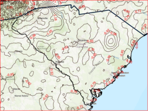
Figure 10 is a plot of GPS on BMS residuals using Geoid16b_NAD depicting large relative differences between stations along the Oregon/Washington State border. It is the near Puget Island along the Columbia River. Station SC0330 and SC1086 are only 7 km apart and the relative difference is -20 cm (-11.4 cm minus 8.6 cm). This could be an issue with the NAVD 88 network design because there doesn’t appear to be many river crossing along the river between border stations. The fact that the residuals on the Washington State side are negative and the Oregon State side are positive is an indication that the stations need to be investigated.

The last figure, figure 11, is a plot of the GPS on BMS residuals using Geoid16b_NAD model that depicts large negative residuals north of the border between Oregon and Washington and positive (or small negative) residuals south of the border. This plot shows that the northern side of the river has large negative residuals all the way to the Pacific Coast. Once again, this is an indication that this portion of the NAVD 88 network should be investigated.
This column has focused on analyzing NGS’ GPS on BM data set that is used to make NGS’ hybrid geoid models. It provided procedures that users could employ when analyzing the differences between the modeled geoid values and the computed geoid values using GPS/Leveling data. This GPSBM data set or one similar will be used to make the next hybrid geoid model, as well as provide input to the transformation model between NAVD 88 and the new 2022 Vertical Reference System. All geospatial users should help develop this GPS on BMS data set to help improve the National Spatial Reference System and future hybrid geoid models. This column provided several examples of large relative differences in residuals between neighboring stations. Each example represents stations that should investigated based on different reasons, such as a weak NAVD 88 leveling network design in the region, the station’s published height attribute code implies that the station was not rigorously adjusted into the NAVD 88, and station pairs have different adjustment dates indicating a possible adjustment distribution correction issue or movement.
NGS has a program called “GPS on Bench Mark” to support users that occupy bench marks with GNSS equipment. This web site contains a lot of good information and provides the users with methods to recover, observe, and report information about stations in NGS’ database. The write up from the webpage is given below. I have highlighted a few sentences that the reader may find useful.
| Write up from: GPS on Bench Marks?
What is GPS on Bench Marks? Improve the National Spatial Reference System (NSRS): Recover: Look up the description of an existing bench mark and visit the bench mark of your choice. Where? Currently there are over 400,000 bench marks across the Conterminous United States (CONUS), Alaska, Hawaii and all U.S. territories. Tidal marks and bench marks are used for determining heights. Use the maps to prioritize which bench marks to observe. Who can participate? Anyone with Global Positioning System (GPS) enabled phones, hand held devices or survey-grade GPS receivers can participate. Recommended procedures vary depending on the type of equipment used. When should I start? You can collect and share information any time. Join volunteer efforts across the United States in celebration of National Surveyors Week beginning March 20, 2016. Contact the local National Society of Professional Surveyors chapter or your NGS geodetic advisor to learn about projects being planned in your local area. How? For specific information on how to help please visit the Recover, Observe, and Report web pages that have instructions. Other resources include “Hunting for Marks!” and Geocaching Benchmark Hunting. Why does this matter? By providing GPS on benchmarks today you can help NGS improve the next hybrid geoid model, increasing access to NAVD 88, and enabling conversions to the new vertical datum in 2022. You can also help the local surveying community know about nearby marks by improving scaled horizontal positions and updating the mark condition or description by submitting a mark recovery. What happens next? NGS will use your data to update its databases and improve future models and tools. If you still have questions, contact the GPS on BM Team. |
In addition to participating in the NGS’ GPS on Bench Mark program, all geospatial users should participate in NGS’ 2017 geospatial summit, which will be held in April in Silver Spring, Maryland.
This summit is an opportunity for all users of the National Spatial Reference System (NSRS) to obtain a better understanding of NGS’ plans to modernize the NSRS. Users will be able to provide feedback directly to NGS leadership. My next column will address NGS plans to replace the North American Vertical Datum of 1988 in 2022.