A depiction of the United States geoid. Areas in yellow and orange have a slightly stronger gravity field as a result of the Rocky Mountains.
No audio available for this content.
Part 1 of this column appeared in the June Survey Scene newsletter, Part 2 appeared in the August newsletter. Upcoming Survey Scene newsletters will carry additional columns in this series.
Basic Understanding of Scientific and Hybrid Geoid Models
David B. Zilkoski
In my first newsletter column of this series, I discussed the basic concepts of GNSS-derived heights. I discussed the three types of heights involved in determining GNSS-derived orthometric heights: ellipsoid, geoid and orthometric.
In my second column (Part 2), I discussed guidelines for detecting, reducing, and/or eliminating error sources in ellipsoid heights. The column focused on guidelines for establishing accurate ellipsoid heights in a local geodetic network.
This column, Part 3, will describe the differences between a scientific gravimetric geoid model and a hybrid geoid model, and why it is important to use both geoid models in your analysis. The latest published United States National Geodetic Survey (NGS) hybrid geoid model, Geoid12B, is made consistent with the United States National vertical height reference frame, that is the North American Vertical Datum of 1988 (NAVD 88). This means a user will be consistent with NAVD 88 when using GEOID12B to estimate GNSS-derived orthometric heights. However, this doesn’t guarantee that your GNSS-derived orthometric heights are accurate.
NGS’ new Beta experimental geoid height models xGEOID14B and xGEOID15B are not distorted to fit the published NAVD 88 heights so they are useful for identifying valid NAVD 88 bench marks (that is, ensuring the monuments haven’t moved since their last survey and their published heights are still valid). Therefore, it is extremely important to validate all NAVD 88 height constraints used to estimate accurate GNSS-derived orthometric heights. Understanding NGS’ scientific and hybrid geoid models will help the user perform the appropriate analysis to determine which leveling-derived orthometric height constraints should be used as constraints. This newsletter will focus on differences between geoid models in a local project area.
Information on NGS’ experimental geoid models can be found here.
Thursday, August 20, 2015
Yearly Experimental Geoid Model Available for Public Review
In 2022, NGS will replace the current North American Vertical Datum of 1988 with one that is based on the geoid — a model of global mean sea level that is used to measure precise surface elevations. NGS created and released annual experimental models of the geoid starting in 2014. This year’s models, xGEOID15A and xGeoid15, are now available for public comment on the NGS beta website. The annual experimental models include new data from the Gravity for the Redefinition of the American Vertical Datum project, which has systematically collected airborne gravity data across the nation since 2008. For more information, contact: Steven.Vogel@noaa.gov
A depiction of the United States geoid. Areas in yellow and orange have a slightly stronger gravity field as a result of the Rocky Mountains.
While we often think of the earth as a sphere, our planet is actually very bumpy and irregular.
The radius at the equator is larger than at the poles due to the long-term effects of the earth’s rotation. And, at a smaller scale, there is topography—mountains have more mass than a valley and thus the pull of gravity is regionally stronger near mountains.
All of these large and small variations to the size, shape, and mass distribution of the earth cause slight variations in the acceleration of gravity (or the “strength” of gravity’s pull). These variations determine the shape of the planet’s liquid environment.
If one were to remove the tides and currents from the ocean, it would settle onto a smoothly undulating shape (rising where gravity is high, sinking where gravity is low).
This irregular shape is called “the geoid,” a surface which defines zero elevation. Using complex math and gravity readings on land, surveyors extend this imaginary line through the continents. This model is used to measure surface elevations with a high degree of accuracy.
How Does the U.S. National Geodetic Survey Generate a Geoid Model?
Generating geoid models is a fairly complex process and is performed by individuals with expertise in physical geodesy and geophysics. It is too complex of a topic for this newsletter but the following excerpt from an NGS publication by Dan Roman provides a good overview of NGS’ process.
Development of the North American Gravimetric Geoid: Adapting the Process to Determine a Unified Central American Geoid
D.R. Roman National Geodetic Survey, 1315 East-West Highway, Silver Spring, MD, USA, 20910
2 Data & Process Improvements
Techniques discussed here have already been addressed previously in Roman and Smith (2001) and Smith et al. (2001), hence only a summary of the approach discussed in those papers is given here. Essentially, the approach currently under investigations seeks to take advantage of recent and pending gains in various data sets related to the gravity field and significantly reduce approximations considered acceptable in the past.
The first thing to consider is the justification for using a geoid over a quasi-geoid, or more accurately, orthometric heights over normal heights. Convincing arguments have been made for orthometric heights (Holdahl 1984) and normal heights (Heiskanen and Moritz 1967). While orthometric heights require extensive knowledge of the gravity field, it is just that reason that warrants their use. Given the extensive knowledge and available data sets, it is incumbent on governmental agencies to generate such models. With a model of the gravity field from the surface to the geoid at hand, anyone subsequently desiring to transform from orthometric to normal heights need only apply it. However, if normal heights are developed and orthometric heights are later desired, the development of such a model will then be required. Clearly, this is a task best suited to national and international organizations that have access to such data and methods. It should not be left to those researchers desiring to use height models in their studies that may not have access to sufficient resources to accomplish this.
With that understanding then, the development of a gravimetric geoid model follows as a mechanism to readily convert between ellipsoidal and orthometric heights. The method summarized here seeks to break the gravity field into three components and solve them separately. In fact the long wavelength component will be derived from a global reference gravity model. The short wavelength will be determined from the terrain. Both of these components will be removed from available gravity observations, which will then reflect the intermediate wavelength signal. A flowchart depicting the determination of these three signals and the generation of a gravimetric geoid is given in Figure 1. Paths shown in red highlight the use of the reference model, paths in green show the determination of the terrain effects, while paths shown in purple highlight the main path to determining Helmert anomalies and then a gravimetric geoid model.
Fig. 1 Determination of a gravimetric geoid using Helmert anomalies.
The expected accuracy of global gravity models in the near future is expected to vastly improve with commission errors below 1-2 cm at wavelengths of 200-300 km (Tscherning et al. 2000). Use of a remove and restore technique (Bašiæ and Rapp 1992) will then result in significantly reduced errors in the residual signal that will be manipulated.
The approach discussed in Roman and Smith (2001) develops the North American gravimetric geoid by removing the terrain effects, downward continuing the residual values, and then restoring the effects of the condensed terrain to generate Helmert anomalies (Heiskanen and Moritz 1967).
To this end, the gravitational attraction of the terrain (TgP) will be calculated and removed from the gravity observations. It will be split into inner and outer zones to reduce computation times. Smith et al. (2001) showed that the effects of using FFT to determine gravitational attraction and potential for both condensed and 3D masses is negligible beyond about a 4 degree cap radius from the point of interest (P). Inside that zone, DEM’s are employed to capture the spherical relationships between the points and more accurately determine the attraction. With available or pending 1 and 3 arc-second DEM’s (Smith and Roman 2001a, NIMA 2001), the signal that may be determined is limited mainly by the computational facilities available to a researcher.
Additionally, the DEM’s will be used to construct grids for the attraction and potential of the condensed terrain (cgPo and cWPo), as well as the potential of the actual terrain (TWPo), all on the geoid. This will capture the short wavelength gravity signal represented by the terrain to the resolution of the grid generated and facilitate later incorporation of this signal into Helmert anomalies.
The resulting point values should be composed mainly of intermediate features in the gravity field with sources deriving from variations in the Moho depth and lateral density variations. This signal should be sufficiently smooth to reduce errors resulting from downward continuation. It should also sufficiently sample the intermediate field to permit the use of minimum curvature (Smith and Wessel 1990) to generate a grid at the same interval as that of the above terrain effects.
Once these terrain effects are restored, these extremely high resolution grids represent residual Helmert anomalies and may be processed using the Stokes integral to determine a best fitting residual gravimetric geoid. Adding the reference geoid derived from the selected global coefficient model will create an equally high-resolution regional gravimetric geoid model.
For a specific country, GPS-derived ellipsoid heights at leveled bench marks (GPSBM’s) provide control information for generating a hybrid geoid model that can be used to specifically, easily, and accurately transform heights between ellipsoidal and orthometric heights (Smith and Milbert 1999, Smith and Roman 2001b).
What are Hybrid Geoid Models and how are they Generated?
NGS’ hybrid geoid model GEOID12B is computed based on the gravimetric geoid USGG2012. As described above, the gravimetric geoid is computed using the satellite model (GOCO3S), terrestrial gravity data, and the altimetric gravity anomaly over oceans. The heights of USGG2012 represent an equipotential surface relative to the reference ellipsoid. The differences between USGG2012 and the zero height surface of NAVD88 are represented by NAD 83 (2011) GNSS-derived ellipsoid heights on NAVD 88 published benchmarks (GPSBM data). See article by Milbert, D.G., 1998: “Documentation for the GPS Benchmark Data Set of 23-July-98,” IGeS Bulletin N. 8, International Geoid Service, Milan, pp. 29-42.) for a excellent description of NGS’ GPSBM dataset.
Currently, the USGG2012 is fitted to the GPSBM data by using the method of least squares collocation. (See section labeled “Excerpts from NGS’ Geoid 12 Web Page” for specific details on how NGS generated hybrid geoid model GEOID12B.) Areas where there are no GNSS observations on published NAVD 88 benchmarks are filled in by USGG2012 geoid. This means a user will be consistent with NAVD 88 when using GEOID12B to estimate GNSS-derived orthometric heights. Being consistent with NAVD 88 is important but being consistent doesn’t guarantee that your GNSS-derived orthometric heights are accurate. The documentation of GEOID12B states that “The relative accuracy of GEOID12B to NAVD88 is characterized by a misfit of +/-1.7 centimeters nationwide.” However, if a published NAVD 88 height used in the development of the hybrid geoid model isn’t valid, then the model is precise but not accurate. That’s why it is important to ensure the monuments used in hybrid geoid models haven’t moved since their last survey and that their published heights are still valid. We will discuss this in more detail later in this newsletter.
Hybrid geoid model, GEOID12B is computed based on the gravimetric geoid USGG2012 . More specifically, they are computed using the satellite model GOCO3S, terrestrial gravity data, and the altimetric gravity anomaly over oceans. The heights of USGG2012 represent an equipotential surface relative to the reference ellipsoid. The differences between USGG2012 and the zero height surface of NAVD88 are represented by GPSBM data.
Currently, the USGG2012 is fitted to the GPSBM data by using the method of least squares collocation. That implies that the voids or empty areas where there are no GPSBM data are filled in by USGG2012 geoid.
There are over 500,000 leveled marks and 80,000 GPS marks over U.S. territory. Of those, there are only 26,000 GPSBM, with half of them concentrated in 5 states. The data density is uneven and sparse in some states. Lists of GPSBMs can be downloaded from the GEOID12B home page.
The GPSBM data provide the geoid height ‘N’ by differencing the ellipsoidal height ‘h’ from the orthometric height ‘H’:
N = h – H
The difference between the geoid height N and that of USGG2012 is computed at every GPSBM. Then, a mathematical model using Least Squares Collocation (LSC) fitting Gaussian functions to describe the behavior seen at the GPSBM is developed. Figure 1 shows empirical data versus the model.
Figure 1: Covariance functions of the geoid differences between USGG2012 and GPSBMs.
Once the relationship between the points is modeled, the model is used to generate a regular grid for interpolation purposes. Figure 2 shows the final conversion surface. This surface represents the difference between NAVD 88 as a datum and the geopotential (geoid) surface used in the gravimetric geoid and is representative of what the datum transformation surface will be when the new geopotential datum is released in 2022. (Similar to VERTCON, which transforms heights from NGVD29 to NAVD88.)
Figure 2: GEOID12B conversion surface.
Summary and Recommendations
Three hybrid geoid models GEOID12, GEOID12A, and GEOID12B are created. They are very similar, but have distinctive differences in few areas. GEOID12A differs from GEOID12 in that it does not use GPSBM data collected in the southern tier states along Gulf Coast, while GEOID12B differs from GEOID12A only in Puerto Rico.
Data in the database are constantly updated, hence older geoid models do not reflect the newer data. To guarantee data consistency, latest model should be used. At this time, GEOID12 and GEOID12A should be superseded by GEOID12B.
Use data conversion outside the GPSBM data areas with caution. Significant extrapolation errors are expected in areas where there are no GPSBM data.
The relative accuracy of GEOID12B to NAVD88 is characterized by a misfit of +/-1.7 centimeters nationwide.
As previously stated, NGS released its latest gravimetric geoid model, xGEOID15. This site will allow the user to compare geoid heights from GEOID12B, USGG2012, xGEOID14 and xGEOID15. (See an example of an input and an output file below.) There are some limited features to this tool. It only provides the results in IGS08 and you are limited to the number of coordinates you can submit at once (20 stations).
Saying that, this tool can be useful for identifying valid NAVD 88 published monuments to be used in the development of future hybrid models. More importantly, it can be used to identify monuments that should NOT be used in future hybrid geoid models or used as constraints in GNSS survey project adjustments.
First, let’s look at the hybrid geoid model GEOID12B values compared with computed geoid height values using the equation N (Computed Geoid Height) = [h (NAD 83 (2011) Ellipsoid Height) – H (NAVD 88 Orthometric Height)]. Table 1 lists the differences between the modeled GEOID12B values and the computed geoid height values for a few stations in an area in eastern North Carolina. Figure 1 depicts the stations locations and values. Many of the differences are less than 1.5 cm which is consistent with NGS’ documentation of GEOID12B that states “The relative accuracy of GEOID12B to NAVD88 is characterized by a misfit of +/-1.7 centimeters nationwide.” However, what is important to notice is that two stations have large differences; station LILIPUT’s difference is 7.4 cm and station BR 7’s difference is -4.6 cm (See highlighted rows in table 1 and boxed area on figure 1). This means that the relative difference between stations LILIPUT (EA0875) and BR 7 (EA0873), which are only 3.3 km apart, is 12.0 cm. This is a large difference and may be indicating a large error in the ellipsoid height and/or the orthometric height at station LILIPUT (EA0875) or station BR 7 (EA0873). In the second newsletter we highlighted that stations LILIPUT and BR 7 were only 3.3 km apart but were not simultaneously observed during the same session. Since the relative difference is 12 cm, the ellipsoid heights of these two should be investigated. It should also be noted that the difference between stations BR 7 (EA0873) and TOWN CREEK (EA0883) is only 3.2 cm. This implies that station B 7 (EA0873) is consistent with some of its neighbors. In the second newsletter we noted that stations B 7 (EA0873) and TOWN CREEK (EA0883) were simultaneously observed during the same session. This may be an indication that B 7 is stable relative to its neighbors and that the orthometric and/or the ellipsoid height of station LILIPUT needs to be investigated.
So what does this mean to the user? If the user establishes a GNSS-derived orthometric height near station LILIPUT using GEOID12B, their results will disagree with the published NAVD 88 heights to around 7 cm; if they establish a GNSS-derived orthometric height near station BR 7, they will disagree with published NAVD 88 heights to around –5 cm. This could also mean that the results in a project could really disagree by more than 7 cm if station LILIPUT moved since its last survey. At this moment, we don’t have enough information to determine if the ellipsoid height or the orthometric height is the problem, or which station may have moved since its last survey.
Table 1. Geoid Height Comparison using GEOID12B Hybrid Model Values.Figure 1. Geoid12B minus Computed Value on NAVD 88 Benchmarks.
Next, let’s look at the differences using the experimental geoid models which are not distorted to be consistent with the NAVD 88 published heights. There will be a bias and a tilt between the systems but in this small areal extent the tilt should not be significant to our analysis. The bias can be removed by looking at relative differences between stations. Table 2, titled “Geoid Height Values for Various NGS Models using xGeoid15 Web Tool,” provides the modeled geoid height minus the computed geoid height where N (Computed Geoid Height) = [h (IGS08 Ellipsoid Height) – H (NAVD 88 Orthometric Height)]. Figure 2, titled “Various Geoid Models minus Computed Geoid Height,” depicts the differences between the various experimental models and computed geoid heights.
Table 2. Geoid Height Values for Various NGS Models using xGeoid15 Web Tool.Figure 2. Various Geoid Models minus Computed Geoid Height.
What is important to note is that stations LILIPUT (EA0875) and WATERWAY (EA0665) seem to be outliers compared to the other stations in the area of study (red boxes on figure 2); and station B 7 (EA0873) seems to be consistent with its neighbors (yellow box on figure 2). For example, station LILIPUT (EA0875)’s residual using xGeoid15B is 25.5 cm and station BR 7 (EA0873)’s residual using xGeoid15B is 13.1 cm, a relative difference of 12.4 cm. Similarly, station TOWN CREEK (EA0883)’s residual using xGeoid15B is 16.3 cm and station BR 7’s residual is 13.1 cm, a relative difference of only 3.2 cm. In my opinion, station LILIPUT (EA0875) needs to be investigated to determine if it has moved since it was last surveyed. In addition, stations east of LILIPUT (EA0875) such as WATERWAY (EA0665) should also be investigated for an ellipsoid and/or orthometric height issue. As previously mentioned, it is also important to note that station BR7 (EA0873), the box in yellow, appears to be consistent to the 3 cm level with its westerly neighboring stations (the boxes in green). This is important to note because the hybrid geoid model could be significantly difference around stations LILIPUT and BR 7 if station LILIPUT was not used in the development of the hybrid geoid model. I am not suggesting that NGS did anything incorrect by including these stations. The goal of the hybrid geoid model is to be consistent with published NAVD 88 values. Unless there is enough information to determine that a station has moved since the last time it was surveyed, the station should be included in the hybrid model. This is where the user may be able to help NGS. If users would investigate outliers like LILIPUT and BR 7 and provide new GNSS survey data and/or leveling data, NGS may have the appropriate information to determine if the monument should be included in the hybrid model.
Part 2 in this Survey Scene series discussed procedures which need to be followed to detect, reduce, and/or eliminate error sources to estimate accurate GNSS-derived ellipsoid heights. This column, Part 3, discussed why a user should understand the differences between NGS’ scientific gravimetric geoid model and hybrid geoid models, and why it is important to use both types of geoid models in their analysis. It demonstrated how to use these geoid models and ellipsoid heights to identify potential issues with published NAVD 88 heights.
My next newsletter column will focus on analyzing the NAVD88 orthometric heights in this area. It will provide basic procedures for validating NAVD 88 height constraints used to estimate GNSS-derived orthometric heights.