The effects of vertical movement on NGS’s modernized 2022 NSRS

My February column explained why it is important to account for horizontal movement of marks everywhere, and not just in areas influenced by active crustal movement due to earthquakes such as Southern California.

It provided information about the NOAA CORS Network (NCN) rates of movement based on International Reference Frame of 2014 (ITRF2014) coordinates and horizontal velocity information.  It highlighted reports from the National Geodetic Survey (NGS) that describe models that will facilitate users transferring coordinates between reference frames and dealing with intra-frame movement between marks based on surveys performed at different epochs.

NAPGD2022 orthometric heights will primarily be accessed through GNSS technology.

As I stated in my February column, this is not just a horizontal positioning issue. In this month’s column, I address estimates of vertical movement that will have to be accounted for in the new, modernized National Spatial Reference System (NSRS).

The NGS 2021 revised Blueprint 2, NOAA Technical Report NOS NGS 64 Blueprint for the Modernized NSRS, Part 2: Geopotential Coordinates and Geopotential Datum, addresses the geopotential aspects of the new, modernized NSRS.  The modernized Geopotential Datum will be called the North American-Pacific Geopotential Datum of 2022 (NAPGD2022).  There will be four primary, interrelated time-dependent products of NAPGD2022:

• a global model of Earth’s geopotential field (GM2022)
• regional gridded geoid undulation models (GEOID2022)
• regional gridded deflection of the vertical models (DEFLEC2022)
• regional gridded surface gravity models (GRAV2022).

NAPGD2022 will provide gridded models for North America (that includes CONUS, Alaska, Hawaii, the Caribbean, Canada, Mexico, Central America and Greenland), American Samoa and Guam/Commonwealth of Northern Mariana Islands (CNMI). My previous columns have described the NAPGD2022 in detail.  The revised NOS NGS 64 report mentioned that NAPGD2022 will be built upon ITRF2020.  It states that NAPGD2022 will operate equally well in any of the four new terrestrial reference frames developed as part of the new, modernized NSRS in 2022.

As I stated in previous columns, orthometric heights in NAPGD2022 will be defined through GNSS ellipsoid heights and GEOID2022. This means NAPGD2022 orthometric heights will primarily be accessed through GNSS technology. GEOID2022 will be defined in a manner that best fits global mean sea level at the epoch of NAPGD2022.

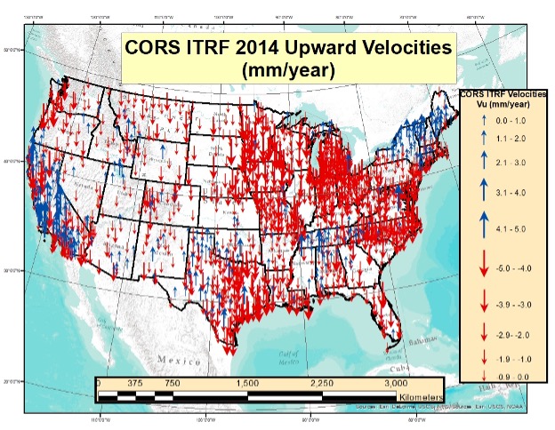
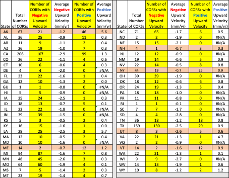
As in my previous column, to better visualize the potential size of the vertical movement, I used the CORS ITRF2014 coordinates and velocities from the NGS website to create plots depicting the upward velocity (Vu) values for CORS that are designated as operational and have computed velocities. [Note: I use the term upward because that is how it is reported on the NGS CORS website under the tab labeled “position and velocity.”  The term upward velocity means movement in both directions — negative is downward and positive is upward.] The box below shows maximum, minimum, average and standard deviations of upward velocity values for each state and territory of the United States.

Table of ITRF 2014 Upward Velocities of US CORSs

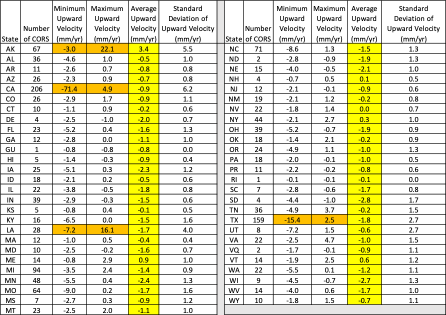
The upward velocity values are not as systematic as the horizontal velocity values, and they are significantly smaller.  I have highlighted the average value velocity column.  As indicated in the table, the values vary from state to state, but they are all small relative to the horizontal movement values. (See my previous column for plots depicting the horizontal values.)

What is interesting is the range of values in some states. For example, Alaska and California have a very large range — understandable because of the active earthquakes and other movement that occur in these states. Also, Louisiana and Texas have a very large range due to local subsidence.

I decided to highlight the values for the conterminous United States (CONUS) in two separate plots.  The box “Upward Velocities (Vu) Between +/–5 mm/year in CONUS” depicts upward velocities (Vu) between +/–5 mm/year in CONUS. The box “Upward Velocities Greater than Absolute Values of 5 mm/year in CONUS” depicts upward velocity values greater than +/–5 mm/year.

Upward Velocities (Vu) between +/- 5 mm/year in CONUS Image: Dave Zilkoski

It’s obvious that most of the vertical movement values are between +/–5 mm/year in CONUS.  There are some large values in California, Louisiana and Texas.  This is highlighted in both plots.

Upward Velocities (Vu) Greater than Absolute Values of 5 mm/year in CONUS (Image: Dave Zilkoski)

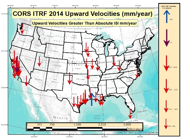
As indicated in the plots, some of the values exceed 10 mm/year. In five years, the heights of marks in these regions could potentially change by 5 cm.  An example of the potential subsidence in the Houston-Galveston, Texas, region is depicted in the box below. As indicated in the plot, some marks are subsiding greater than 2 cm/year.  That means in five years the marks in that region could have subsided more than 10 centimeters.

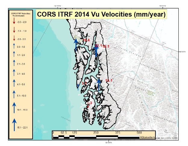
The box below depicts the values in Alaska. Most of these values indicate that the marks are uplifting. Some of these values exceed 10 mm/year. Once again, height coordinates in some regions will potentially change 5 cm in five years. I generated a separate plot for the southeastern region of Alaska. (See the box titled “Upward Velocities (Vu) in Southeastern Alaska.”)

Upward Velocities (Vu) in Alaska [All Values] Image: Dave Zilkoski

Upward Velocities (Vu) in Southeastern Alaska [All Values] Image: Dave Zilkoski

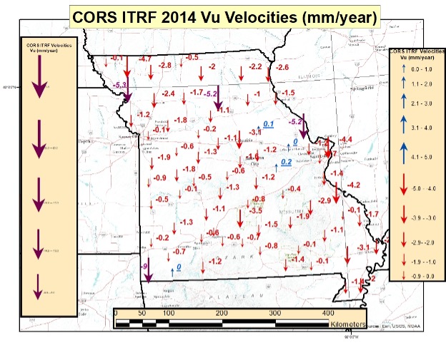
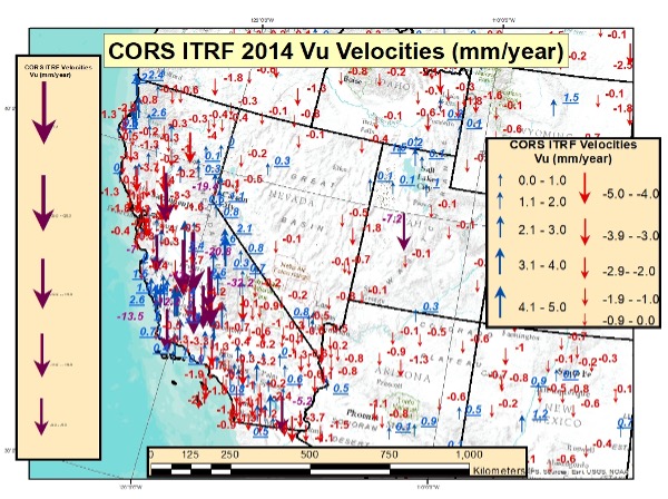
As I did in my previous columns, I prepared several plots that depict the upward velocities in various regions of the United States. See the boxes below for North Carolina, Missouri Southwest U.S. The plots indicate that the magnitude of the vertical movement varies from state to state, as well as within the states.

CORS ITRF 2014 Upward Velocities (Vu) in Missouri [All Values] Image: Dave Zilkoski

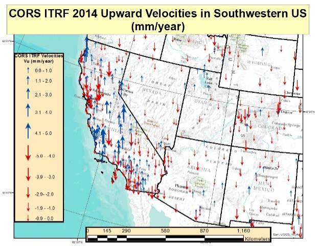
CORS ITRF 2014 Upward Velocities (Vu) in Southwest U.S. [All Values] Image: Dave Zilkoski

CORS ITRF 2014 Upward Velocities (Vu) in Southwest U.S. [Values Between +/- 5 mm/year] Image: Dave Zilkoski

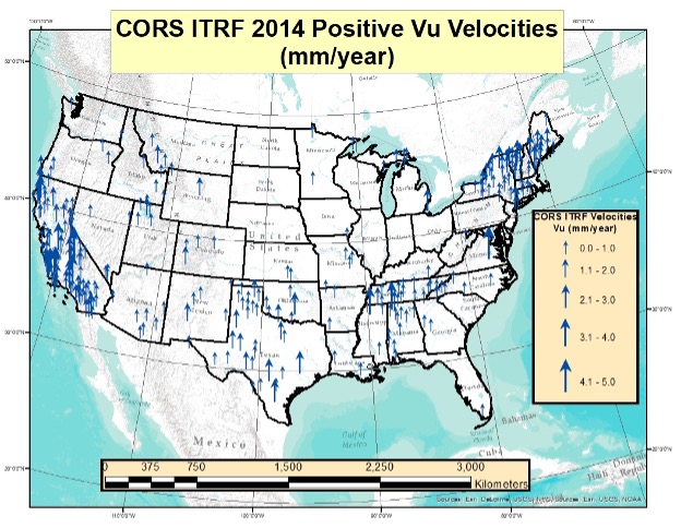
I also generated plots that separately depict the positive and negative upward velocities for the conterminous United States. There are more negative upward velocity values than positive values.

CORS ITRF 14 Positive Upward Velocities (Vu) in Conterminous U.S. (Values between 0 and 5 mm/year) Image: Dave Zilkoski

CORS ITRF 2014 Negative Upward Velocities (Vu) in Conterminous U.S. (Values between -5 and 0 mm/year) Image: Dave Zilkoski

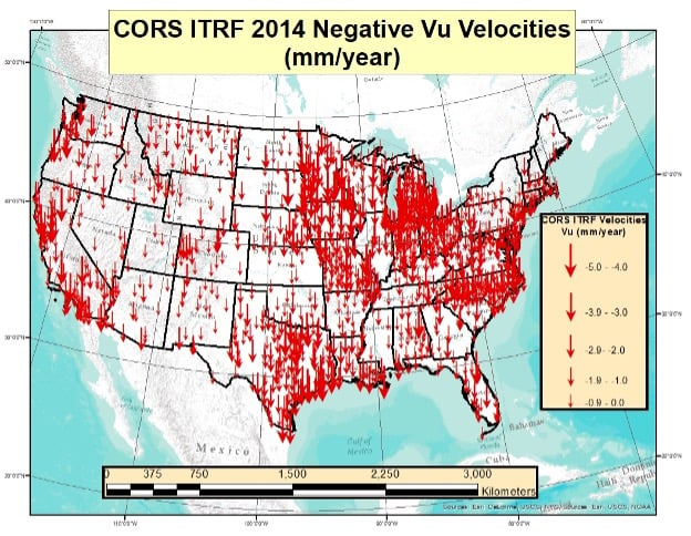
The table below provides the number of CORS with negative upward velocity values and the number of CORS with positive values for every state and territory of the United States. I have highlighted the states and territories that have more positive values than negative values. As you can see, only six states have more positive upward velocities than negative values. Four of the six states are in Northeastern United States.

So far, this column has only addressed the vertical movement at the NCN CORS.  The values at the sites indicate the potential movement of marks in the area of the CORS. The rates are based on GNSS data and have an estimate of error associated with them.

I’m not sure how NGS will address the vertical movement effects in the new, modernized NSRS. That said, NGS will be monitoring the CORS and looking for trends to help describe the movement at the CORS. These trends will be an indication of what may be happening in the area.

In addition to the movement of individual marks, there are geophysical reasons for changes in the geoid. As I stated in previous columns, orthometric heights in NAPGD2022 will be defined through ellipsoid heights and GEOID2022. Therefore, changes in the geoid model will be very important to users estimating orthometric heights using GNSS.

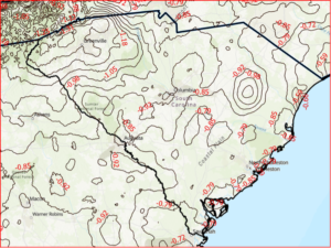
As stated in the NGS 64 report, NGS has set a goal of maintaining geoid accuracy at 1 centimeter (1 standard deviation) in both absolute and differential geoid undulations. Figure 13 from the NGS 62 Report depicts an estimate of the secular change in the geoid. As indicated in the plot, the changes are very small, ranging from –1.25 mm/year to 1.5 mm/year.

What I find interesting is the small negative change in the southeastern United States. There are other drivers for geoid changes. Future columns will address some of these changes and what it means to users.

Figure 13 from NOS NGS 62 Report Image from NGS website: Blueprint 2 Revised NOAA_TR_NOS_NGS_0064.pdf Figure 13 – Secular Geoid Change

Lastly, I’d like to highlight a new service from NGS: “NGS Webinar Series Certificates of Attendance.” See the box titled “Ways to Earn a Certificate of Attendance.” Basically, users can earn certificates by viewing a webinar after it has been posted by NGS.  This is very useful for users who could not attend the original webinar. I encourage all users to check out the site to find out more information about the new service.

Ways to Earn a Certificate of Attendance Image from NGS website: https://geodesy.noaa.gov/web/science_edu/webinar_series/certificates.shtml