How NGS can implement a time-dependent geopotential datum

December 4, 2019 - By David B. Zilkoski

The National Geodetic Survey (NGS) has published a technical report that describes options for how NGS can implement a time-dependent geopotential datum and thus a time-dependent geoid model. My last column described the latest version of NGS’ VERTCON model. As mentioned in the column, NGS is developing these models and tools to support the implementation of the North American-Pacific Geopotential Datum of 2022 (NAPGD2022).

NAPGD2022 is going to be a time-dependent geopotential datum. In other words, the reference geopotential will change over time and therefore the geoid height value will change over time. NAPGD2022 was described in detail in NGS’ publication “Blueprint for 2022, Part 2: Geopotential Coordinates,” and my December 2017 column. Blueprint for 2022, Part 2 states that a gridded geoid model GEOID2022 will be created and it will contain two components:

The first component will be time independent, denoted as the Static Geoid model of 2022 (SGEOID2022).
The second component will be a time-dependent geoid undulation model, encompassing permanent geoid changes greater than or equal to 1 millimeter per year, denoted as Dynamic Geoid model of 2022 (DGEOID2022).

NGS will publish a GEOID2022 value that will be based on both SGEOID2022 and DGEOID2022. As stated in the document, GEOID2022 will be the official zero-height surface for orthometric heights within NAPGD2022, and thus within the NSRS. The box titled “Excerpt from Blueprint for 2022, Part 2, Figure 10-2” is a diagram that describes the process of creating the regional high resolution gridded GEOID2022 model. I have highlighted the GEOID2022 model and its two components, SGEOID2022 and DGEOID2022.

Excerpt from Blueprint for 2022, Part 2, Figure 10-2

Image: National Geodetic Survey

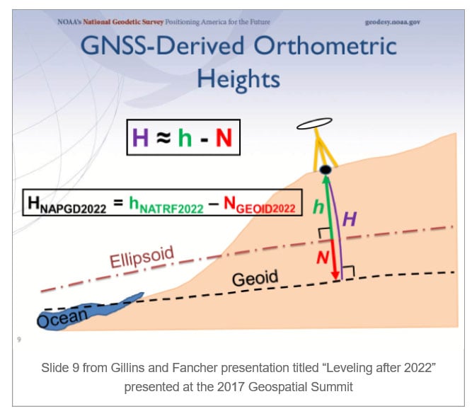
First, it’s important to note the role of the geoid in estimating GNSS-derived orthometric heights. As described in a previous column, GNSS-derived Orthometric Heights are computed using the following formula: orthometric height (H) = ellipsoid height (h) minus geoid height (N). See the box titled “NAPGD2022 GNSS-Derived Orthometric Height.”

NAPGD2022 GNSS-Derived Orthometric Height

Source: Slide 9 from Gillins and Fancher presentation titled “Leveling after 2022” presented at the 2017 Geospatial Summit

So, what does it take to compute a time-dependent geoid model and what is NGS’ plan to accomplish this project The technical report titled “ A Preliminary Investigation of the NGS’s Geoid Monitoring Service (GeMS)” describes options for how NGS can implement a time-dependent geopotential datum and thus a time-dependent geoid model (See box titled “NGS Publishes Report on GeMS”). The report contains too much information for a single column. This column will highlight some of the sections of the report. The document does contain a lot of technical information and I would encourage everyone to download the document.

NGS Publishes Report on GeMS

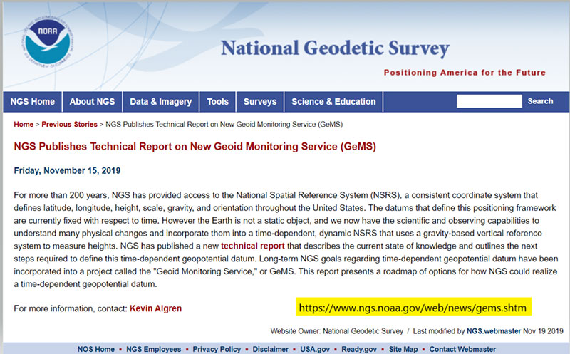
Screenshot: National Geodetic Survey

The technical report describes the current state of knowledge and outlines next steps required to define a time-dependent geopotential datum for the Nation. NGS created a project called “The Geoid Monitoring Service,” or simply GeMS, to accomplish their long-term goal of establishing a time-dependent geopotential model.

The report addressed the following five topics:

A foundational introduction to the various types of geophysical phenomena that are causing both size and shape change to the geoid,
Geodetic observing techniques that are presently available to monitor geoid change,
An objective evaluation of NGS’s current ability to incorporate these techniques into a long-term monitoring service like GeMS,
Known barriers to accomplishing such a project, and
Potential observing techniques that might become available in the next 10-20 years, but are not currently mature enough for operational use.

The document presents a roadmap of options for how NGS could realize a time-dependent geopotential datum, and how NGS can support the dynamic datum into the future with independent validation surveys and datasets.

The report discusses the available geoid monitoring techniques that NGS has to support modeling the changes in the geoid. There are three existing NGS program areas and associated technical expertise that could be utilized in an operational GeMS:

NGS’s Gravity Program,
the NOAA CORS Network, and
GPS/geodetic leveling campaigns.

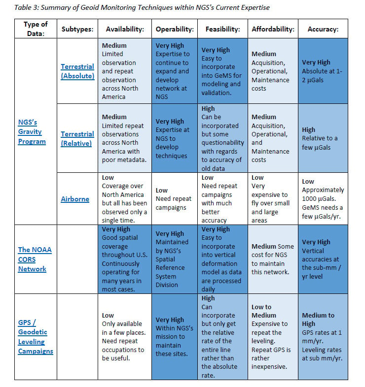
It is noted that individuals these techniques cannot provide 100% of what GeMS requires but combining various programs would be sufficient. The report does a great job of describing these three program areas. The box titled “Summary of Geoid Monitoring Techniques within NGS’ Current Expertise” is Table 3 from the Technical Report. The table list the affordability and accuracy attributes for each of the program areas. NGS’ Gravity Program provides high quality gravity data to internal and external stakeholders. The program provides gravity data required for NGS’s geoid modeling.

Summary of Geoid Monitoring Techniques within NGS’ Current Expertise

Source: National Geodetic Survey

The report provides a good overview of the expertise and instrumentation of NGS’ Gravity Program. The table titled “Summary of NGS’ Terrestrial Gravity Instruments” is a compilation of information on historical methods and instrumentation from the technical report.

Summary of NGS’ Terrestrial Gravity Instruments

: FG5 Absolute Gravimeter. The FG5(X) absolute gravimeter is manufactured by Micro-g LaCoste Inc. in Lafayette, Colorado. It is currently the highest-accuracy, commercially-available absolute gravity meter, with an accuracy of about ±2 μGals. NGS owns and operates instrument number FG5X-102. (Source: National Geodetic Survey)

: A10 Absolute Gravimeter. A field deployable version of the laboratory FG5 absolute gravimeter, was developed by Micro-g LaCoste in the early 2000’s. This instrument, now known as the A10, operates on principals nearly identical to the FG5 free fall gravimeter. However, the laser used in the A10 system is not a primary standard due to the low power and fragile nature of the Iodine based laser, and does need to be calibrated routinely. (Source: National Geodetic Survey)

: Scintrex CG-6 Relative Gravimeter. The Scintrex CG-6 relative gravimeter is the newest generation of the CG line of quartz sensor relative gravity meters. The CG-6 (like its predecessors the CG-3 and CG-5) operates on the same fundamental theory as the LaCoste and Romberg G and D relative gravimeters, but uses a quartz sensor spring instead of a metal sensor. The primary advantage of a quartz sensor is its insensitivity to instrument shock or vibration that can cause offsets in the gravity measurements. (Source: National Geodetic Survey)

: LaCoste and Romberg Relative Gravimeter. LaCoste and Romberg (L&R) relative land, air/sea, borehole, and tidal gravimeters have been manufactured by LaCoste and Romberg Gravity Meters, Inc. since 1959. The company later merged into Micro-g LaCoste, Inc., and the LaCoste land gravimeters were discontinued. Unlike the Scintrex gravimeters, these rely on metal zero-length-springs. (Source: National Geodetic Survey)

: Superconducting Cryogenic Gravimeter. A superconducting cryogenic gravimeter is designed to be continuously monitor relative changes in the local gravity over time. It main applications include precise tidal analysis, ground water monitoring, and geodynamics. The precision of an SG is still unmatched by any other instrument at better than 0.1 μGals at short time scales. (Source: National Geodetic Survey)

: gPhoneX Gravity Meter. The gPhoneX, manufactured by Micro-g LaCoste, is a low (linear) drift, metal spring-based gravimeter. Like the SG, it is designed to measure relative changes in gravity over time, at a fixed location. While not as precise as the SG at short time scales; at periods of longer than a few hours, the noise characteristics of the two instruments are quite similar. The advantages of a gPhoneX compared to a SG for long term monitoring include lower cost, lower power consumption, increased portability, and lack of a requirement for maintaining superconducting temperatures. (Source: National Geodetic Survey)

: JILAg Absolute Gravimeter. The AFGL, JILA/IGPP and JILAg series of absolute gravimeters are the out-of-production predecessors to the FG5 gravity meter. These instruments were developed by James Faller and colleagues beginning in the mid-1970s, and were crucial for defining and providing the basis for the IGSN71, NGSGN, and other scientific projects. Agency (now NGA), the University of California at San Diego (IGPP), and NGS. (Source: National Geodetic Survey)

The document highlights something about the United States gravity data that most users don’t think about. That is, gravity values are referenced to a gravity network just like NGS’ published orthometric heights are referenced to the NAVD 88. In the mid-1950s, a coordinated effort was initiated by the International Association of Geodesy (IAG) to make gravimeter ties throughout collaborating parts of the world to support establishment of an International gravity datum.

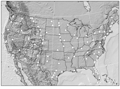
It incorporated intercontinental, north-south, calibration lines and long-distance ties established by airplane. The majority of USA relative gravimeter work was done from 1965 – 1967, resulting in the network shown in the box titled “International Gravity Station Net of 1971 (IGSN71) in CONUS.” The report states that the calculations were completed by Urho A. Uotila of The Ohio State University around 1970.

The gravity network was constrained by a network of ballistic absolute gravimeters. Five of the eight absolute gravimeter sites were in CONUS. It was a world-wide, simultaneous adjustment and published as The International Gravity Standardization Net 1971 (I.G.S.N. 71). A

s of December 2019, the IGSN71 remains the official international gravity datum. Many of these stations have been destroyed over the decades, in particular those at passenger airport terminals.

International Gravity Station Net of 1971 (IGSN71) in CONUS

(Source: Figure 14 from geodesy.noaa.gov)

Figure 14: IGSN71 Gravity Stations. (Source: National Geodetic Survey)

In the mid-1970s, NGS was involved in two major readjustment projects, replacement of NAD27 with NAD 83 and the replacement of NGVD 29 with NAVD 88. At the same time, the NGS gravity group were evaluating the gravity data in NGS database and the gravity stations involved in the IGSN71. During the period 1975 and 1979, NGS and NGA (formally DMA) performed relative gravity surveys around CONUS to evaluate the stations.

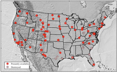
A report by Robert Moose titled “The National Geodetic Survey Gravity Network” published by NGS in 1986 documents the results of the surveys. This network is denoted as the National Geodetic Survey Gravity Network (NGSGN) and depicted in the box titled “National Geodetic Survey Gravity Network (NGSGN) in CONUS.” The NGSGN was constrained by 8 absolute gravimeter stations and consisted of 232 stations. Differences between NGSGN values and IGSN71 values were computed to evaluate or detect change in gravity values.

The box titled “Gravity Differences between NGSGN and IGSN71 Common Stations” depict these differences. The report states “In summary, the gravity differences between NGSGN and IGSN are generally small and many of the larger differences may be due to vertical motion.

National Geodetic Survey Gravity Network (NGSGN) in CONUS

(Source: Figure 15 from geodesy.noaa.gov)

Figure 15: NGSGN Stations. Destroyed stations known as of July 2019. (Source: National Geodetic Survey)

Gravity Differences between NGSGN and IGSN71 Common Stations

(Source: Figure 16 from geodesy.noaa.gov)

Figure 16: Difference between NGSGN and IGSN71 AG values [mgal] (Source: National Geodetic Survey)

The basic rule of thumb for estimating land movement using gravity changes is: 1 meter of change equals 0.3086 mgals (1 cm of change equals 0.003086 mgals). It should be noted that a positive difference in gravity in the figure indicated apparent subsidence. As stated by the 1986 report by Moose, the large difference in Houston-Galveston region is most likely due to subsidence.

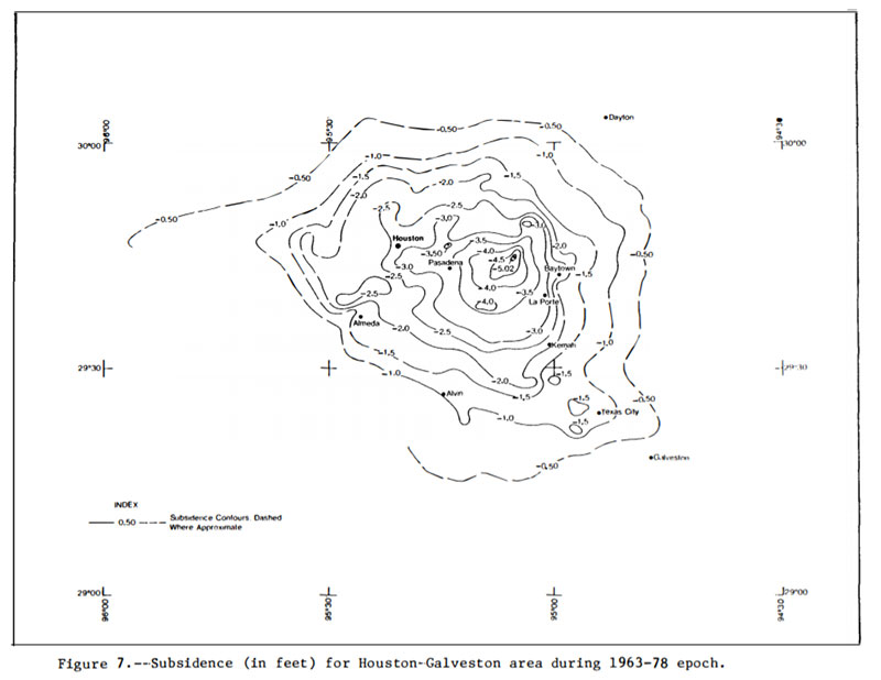
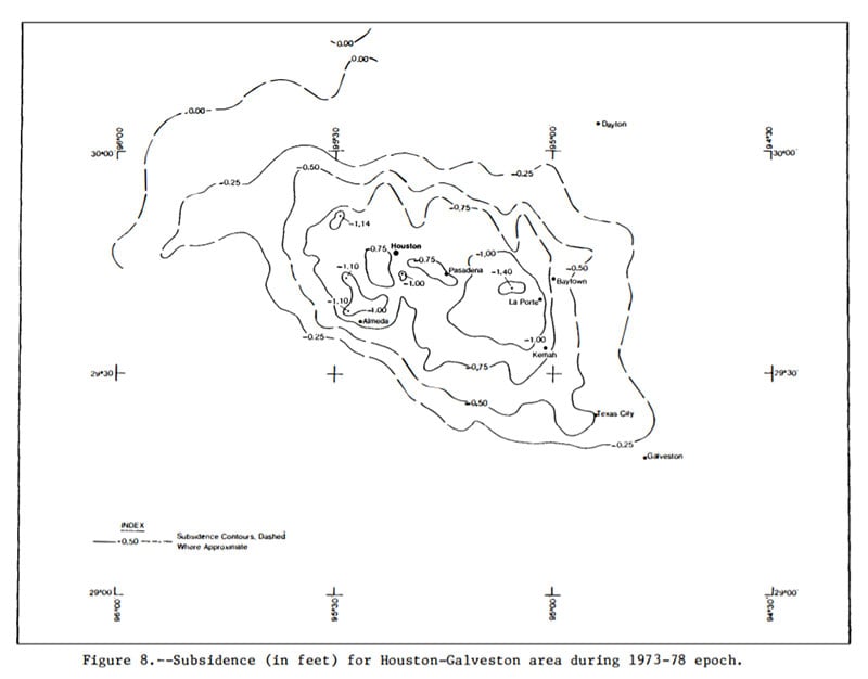
A report documenting the apparent movement in the Houston-Galveston region was published by NGS in 1980. The boxes titled “ Estimate of Subsidence in Houston-Galveston Area During 1963-78 Epoch” and “Estimate of Subsidence in Houston-Galveston Area During 1973-78 Epoch” provide estimates of the movement in the region that include the same epoch of the two gravity networks. These two plots agree with the summary statement in the 1986 report.

Estimate of Subsidence in Houston-Galveston Area During 1963-78 Epoch

(Source: Figure 7 from ngs.noaa.gov)

NOTE: 30 cm approximately equals to 1 foot (Source: National Geodetic Survey)

Estimate of Subsidence in Houston-Galveston Area During 1973-78 Epoch

(Source: Figure 8 from https://www.ngs.noaa.gov/PUBS_LIB/The1978Houston_Galveston_and_Texas_GulfCoast_VerticalControlSurveys_TM_NOS_NGS27.pdf)

NOTE: 30 cm approximately equals to 1 foot (Source: National Geodetic Survey)

What does all this mean to the geoid? Accurate and current gravity data are critical to the development of an accurate geoid model that includes estimating changes in the geoid model over time.

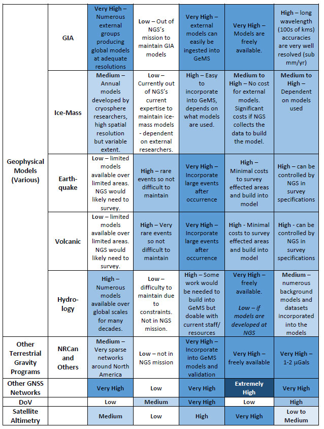
The technical report on NGS’ Geoid Monitoring Service (GeMS) describes geodetic and geophysical techniques that are currently known to NGS and show promise for GeMS (see the box titled “Summary of Known Geoid Monitoring Techniques that are currently outside of NGS’s Expertise). It should be noted that all of these techniques rely on a non-NGS entity to create a product (such as a model or dataset) that NGS can utilize in their products and services. This is nothing new; NGS leverages partnerships for other products such as the GOCO05S satellite gravity model produced by an ESA consortium led by the Technical University of Munich. This model is used by the NGS geoid team in static geoid modeling.

Summary of Known Geoid Monitoring Techniques that are currently outside of NGS’s Expertise

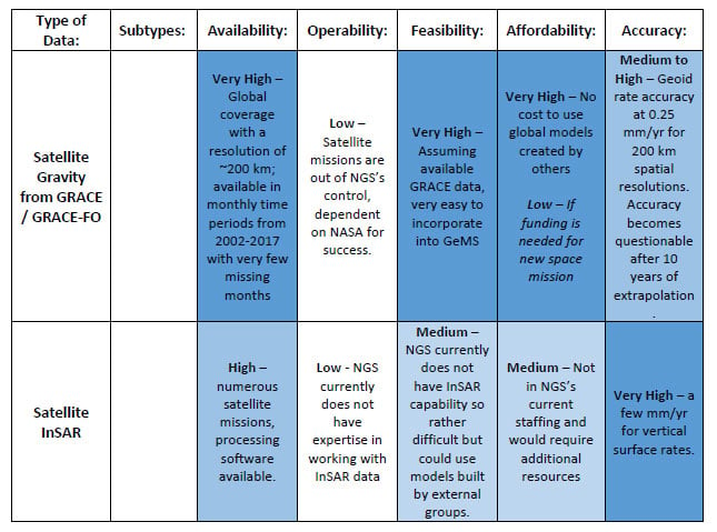
(Source: Table 7 from Technical Report NOS NGS 69)

Continuation of Summary of Known Geoid Monitoring Techniques that are currently outside of NGS’s Expertise

(Source: Table 7 from Technical Report NOS NGS 69)

As apparent by all of the types of data required to monitor the geoid, NGS has a challenging task to establish a Geoid Monitoring Service. Why is it important to invest resources to monitor the geoid? Analyzes of temporal satellite gravity missions provide changes in gravity values that can be use to create changes in the geoid. The GRACE (Gravity and Climate Experiment) satellite mission was designed to provide the temporal gravity field variations throughout its mission (duration 2002 – 2017). There are analysis centers that produce models using the GRACE data – University of Texas at Austin Center for Space Research (UTCSR), NASA Jet Propulsion Laboratory (JPLEM), and GFZ German Research Center for Geosciences (GFZOP). Release 6 denoted as RL06 is the most current GRACE data from these groups.

The data can be used to illustrate the magnitudes and resolutions that GRACE models provide to the seculargeoid rates for CONUS and Alaska. The boxes titled “GRACE Trend over CONUS from UTCSR RL06” and “GRACE Trend over Alaska from UTCSR RL06” are plots from Technical Report NOS NGS 69 that show these secular geoid trends from UTCSR-RL06. The plots indicate very small changes in the geoid but they are significant if the goal is to monitor the geoid model to the mm/year level.

GRACE Trend over CONUS from UTCSR RL06

Figure 27: GRACE Trend over CONUS from UTCSR RL06 Model [mm/yr] (Source: Figure 27 from Technical Report NOS NGS 69)

GRACE Trend over Alaska from UTCSR RL06

Figure 28: GRACE Trend over Alaska from UTCSR RL06 GRACE Model [mm/yr] (Source: Figure 28 from Technical Report NOS NGS 69)

Another product available from various processing centers are surface mass concentrations (mascons) as observed by the GRACE satellites. Once again, these mascons can be used to generate a secular geoid rate. The boxes titled “Geoid rate over CONUS based on the GSFC mascon model” and “Geoid rate over Alaska from GSFC mascon model” are plots from Technical Report NOS NGS 69 that provide the secular geoid rate based on the NASA GSFC mascon model. Once again, the plots indicate very small changes in the geoid but there is a systematic change to the geoid based on the analysis of the data from the GRACE mission.

Geoid rate over CONUS based on the GSFC mascon model

Figure 32 From Technical Report NOS NGS 69: Geoid rate over CONUS based on the GSFC mascon model [mm/yr] (Source: Figure 32 From Technical Report NOS NGS 69)

Geoid rate over Alaska from GSFC mascon model

Figure 33 From Technical Report NOS NGS 69: Geoid rate over Alaska from GSFC mascon model [mm/yr] (Source: Figure 33 From Technical Report NOS NGS 69)

The report stated that when considering monitoring the geoid, the greatest change to the geoid from glacial isostatic adjustment (GIA) processes is centered in northern Canada, but there is “still a significant geoid height trend in the Northern Plains, Great Lakes, and Northeast regions of CONUS.”

It was noted that if GIA processes are not considered, a 1 cm error in the geoid undulation would occur within 18 years. NADGPD2022 orthometric heights are going to be established using a NATRF2022 ellipsoid height and a GEOID2022 geoid height. This is why the geoid needs a time-dependent component.

This column highlighted NGS new Geoid Monitoring Service (GeMS); and, that NGS’ will be publishing a gridded geoid model GEOID2022 that will contain two components:

The first component will be time independent, denoted as the Static Geoid model of 2022 (SGEOID2022) and
The second component will be a time-dependent geoid undulation model, denoted as Dynamic Geoid model of 2022 (DGEOID2022).

NGS will publish a GEOID2022 value that will be based on both SGEOID2022 and DGEOID2022. The column provided examples of how GRACE data can be used to illustrate the magnitudes of secular geoid rates for CONUS and Alaska.