GNSS timing measurements from a low-Earth orbiting satellite

Read Richard Langley’s introduction to this article: “Innovation Insights: What is a CubeSat?”

Figure 1: Bobcat-1, with communications antenna stowed (left) and deployed (right). Bobcat-1 measures approximately 10 x 10 x 30 centimeters. (All figures except FIGURE 3 provided by the authors)

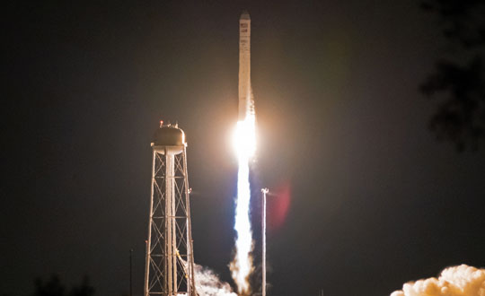
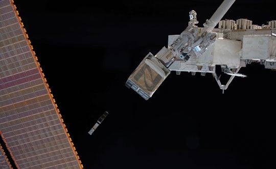
Bobcat-1 was a three-unit CubeSat developed and built at Ohio University’s Avionics Engineering Center in Athens, Ohio, and was named after the university’s mascot. FIGURE 1 shows Bobcat-1 with and without its antenna deployed. The satellite was launched to the International Space Station in October 2020 (see FIGURE 2) and deployed into low-Earth orbit (LEO) the following month (see FIGURE 3). In April 2022, it deorbited and burned up in Earth’s atmosphere as planned, after a successful 17-month mission, lasting eight months longer than anticipated. The last signal decoded from Bobcat-1 was received only about 10 minutes before the satellite’s demise, from an altitude of about 109 kilometers, by an amateur radio operator (ZR6AIC) near Johannesburg, South Africa, associated with SatNOGS, a global network of amateur satellite-networked open ground stations.

The main mission of the Bobcat-1 CubeSat was to evaluate the feasibility of GNSS-to-GNSS time offset monitoring from LEO. One of the secondary mission objectives was GNSS spectrum monitoring.

In addition, Bobcat-1 also included a side-mission, hosting a software-defined GPS/Galileo receiver developed by the University of Padova and Qascom — an Italian engineering company providing security solutions in satellite navigation and space cybersecurity — to perform its in-space demonstration and testing. This receiver served as a prototype for the receiver soon to be launched on NASA’s Lunar GNSS Receiver Experiment (LuGRE) mission.

Communications and control of the satellite utilized the 70-centimeter amateur radio satellite band (435-438 MHz) at a typical data rate of 60 kilobits per second and were primarily conducted using a dedicated ground station on the roof of the engineering building at Ohio University (see FIGURE 4). In total, Bobcat-1 collected and downlinked more than 656 megabytes of data during its lifetime. Over the course of the mission, Bobcat-1’s firmware was updated in-orbit on six occasions, allowing for minor enhancements to the data collection system.

Figure 2: Bobcat-1 launches aboard the Cygnus NG-14 resupply mission to the International Space Station. (All figures except FIGURE 3 provided by the authors.)

BACKGROUNDS: GNSS-TO-GNSS TIME OFFSET

GNSS-to-GNSS time offsets — also referred to as GNSS inter-constellation time offsets, inter-system biases or XYTOs — are among the critical parameters for full GNSS interoperability. Users with poor GNSS visibility, such as high-altitude spacecraft, which operate above the GNSS constellations, often do not have enough satellites in view to enable an accurate solution and can experience high dilution of precision. These users could benefit from XYTO estimates provided externally, assuming their receiver-characteristic inter-system biases (ISBs) are calibrated.

To determine a user solution using measurements from a single GNSS constellation, one must solve for four unknown parameters: the user’s spatial coordinates and the receiver-to-system time offset. This means that a minimum of four satellites must be visible to solve for a user solution. If a user has sufficient visibility of satellites from different constellations, a multi-GNSS solution can be determined. However, when applying measurements from multiple constellations, an additional unknown is added for each constellation used. For example, for a user solution incorporating measurements from both GPS and Galileo, one needs to solve for five unknowns: the user’s spatial coordinates, the receiver-to-GPS time offset, and the receiver-to-Galileo time offset. Since each constellation’s time scale is independent of the others, the inter-system time offset between the time scales leads to a prominent bias in a multi-constellation solution. Inter-system time offsets between GPS, Galileo, GLONASS, and BeiDou are generally expected to range from 10 to 100 nanoseconds, resulting in 3 to 30 meters of possible positioning error.

System-to-system time offsets are currently estimated by extensive networks of ground stations, such as those used by the International GNSS Service Multi-GNSS Experiment (MGEX). In addition, GNSS service providers often broadcast XYTO estimates in their navigation messages.

Figure 3: Bobcat-1 is deployed into low-Earth orbit by the Nanoracks CubeSat Deployer alongside SPOC, a CubeSat developed by the University of Georgia. (Photo: NASA)

So, why would estimating XYTOs from LEO be of interest?

Low-Earth orbit enables high GNSS visibility. The approximately 90-minute orbital period allows for observations from nearly all GNSS satellites multiple times per day. This enables high visibility of multiple satellites from each constellation, in turn enabling high observability of constellation parameters such as XYTOs, leveraging satellite-characteristics errors. In addition, tropospheric errors are absent and multipath is limited and can be bounded based on the CubeSat’s dimensions and geometry. Exploiting measurements from LEO could provide additional measurements and independent monitoring of the XYTO estimates provided by ground networks.

However, to estimate system-characteristic XYTOs, the receiver-characteristic biases need to be calibrated. The target is to reach accuracy of approximately 1 nanosecond or possibly lower. Therefore, the error sources need to be evaluated, mitigated, or bounded.

Figure 4: Bobcat-1’s dedicated ground station on the roof of Stocker Center in Athens, Ohio. (All figures except FIGURE 3 provided by the authors.)

Although the ionospheric effects are lower in LEO than on Earth, they cannot be neglected. Therefore, dual-frequency ionospheric delay estimates must be applied. To do so, the receiver’s inter-frequency biases (IFBs), which can introduce errors on the order of nanoseconds, need to be calibrated, as well as the satellite differential code biases (DCBs), orbit and clock errors and receiver antenna group delay. An additional challenge introduced by the LEO environment is the wide range of temperatures to which the receiver is subjected. Over a single orbit, the receiver’s temperature can vary from approximately 0 to 50 degrees Celsius. The effects of these temperature variations cause fluctuations in the receiver’s IFBs, which need to be evaluated and calibrated. Pre-launch measurements in a controlled environment using a climate chamber and two receivers of the same make and model were used for calibration. We have detailed those measurements elsewhere.

The multipath error can be bounded, as a first approximation, to 10 centimeters (or about 0.3 nanoseconds in equivalent signal delay) due to the dimensions of the CubeSat. However, given the mount of the antenna is on one of the CubeSat’s two 10 × 10 centimeter faces, that upper bound is in practice much smaller and the multipath error is mostly negligible.

Finally, the last remaining major error sources to be calibrated are the receiver ISBs. The main goal, to demonstrate the feasibility of LEO-CubeSat-based monitoring of GNSS XYTOs, requires showing the stability (or the repeatability) of the receiver biases in orbit.

Table 1: Summary of data collections discussed in this article.

DATA COLLECTION

Bobcat-1’s primary payload was a NovAtel OEM719, a triple-frequency multi-GNSS receiver, enabling measurements on all frequencies from GPS, GLONASS, Galileo and BeiDou, as well as the regional navigation satellite systems (RNSSs) QZSS and NavIC. The measurements were collected and downloaded, for post-processing purposes.

Pseudorange and carrier-phase measurements, as well as carrier-to-noise-density ratio estimates, were collected, together with the receiver’s position and velocity estimates, and other parameters such as the temperature measured by the two sensors embedded in the receiver. In limited instances, power spectral density measurements and in-phase and quadrature (I/Q) component samples were collected to support the secondary mission, GNSS spectrum monitoring. The limited downlink capacity of the satellite constrained these measurements to short time intervals.

Figure 5: Number of observations recorded by Bobcat-1 from each GNSS constellation during a data collection started on February 27, 2022.

The goal of the mission is to estimate the XYTOs for all the GNSS constellations. However, in this article only the Galileo-to-GPS time offset (GGTO) is considered. The Galileo Performance Reports published by the European Union Agency for the Space Programme (EUSPA) provide information on the accuracy of the GGTO broadcast parameters, which are typically within approximately 3 nanoseconds of the true GGTO. Therefore, the broadcast GGTO provides a point of comparison and reference for Bobcat-1’s estimates.

A summary of the data collections considered in this work is provided in TABLE 1. These data collections are among the longest recorded by Bobcat-1. As an example, FIGURE 5 shows Bobcat-1’s data collection for February 27, 2022. It should be noticed that data collections were initiated from the control station at Ohio University when the CubeSat was in view, and each data collection would start only when the satellite’s battery voltage was above a defined threshold. The collection would stop safely if a minimum voltage threshold was reached. The data sets collected during the first months of the mission had durations limited to one to four hours, since the minimum battery voltage threshold was set conservatively. However, as the mission continued, data collections recorded in the last several months before deorbiting were configured with lower thresholds, enabling continuous data collections with durations of up to 24 hours. During the longer data collections, the sampling period was set to 20 seconds to reduce the total quantity of data stored and downlinked. The work described here focuses on a select few data collections that span a period of five months between September 28, 2021, and February 27, 2022.

Figure 6: Bobcat-1’s ground track during a data collection for XYTOs estimation held in February 2022, approximately 24-hours long. Note that the blue dots correspond to the positions (latitude and longitude) of Bobcat-1. The red stars indicate that even if the position was calculated thanks to a multi-frequency and multi-GNSS solution, GPS L1 C/A measurements were not available. Analysis of the carrier-to-noise-density ratio measurements and comparison with the available spectrum measurements showed that in correspondence to those positions interference was present.

The data contain multi-frequency measurements from all systems, with an average of 180 observations made per sample. The maximum number of observations at once was 217. While multi-frequency measurements were collected from all constellations, this analysis only uses single-frequency measurements from two constellations: GPS L1 C/A and Galileo E1C.

RESULTS

There are two simple approaches to calculating inter-constellation time offsets: one involves computing multiple single-constellation user solutions, and the other involves a single multi-constellation user solution. Each approach has slightly different effects in terms of error propagation. In the first approach, the XYTOs can be calculated by taking the difference of the independently calculated receiver-to-system time offsets. This method requires at least four satellites from each constellation to be visible. In the second approach, all the receiver-to-system time offsets for all constellations involved in the solution are solved simultaneously. This reduces the number of measurements required per-constellation, with the minimum number of measurements needed being equal to the number of unknown state variables.

Figure 7: Broadcast GGTO (red) compared to Bobcat-1 Galileo-GPS time offset estimate, before calibration (blue) and filtered estimate (black). The results are related to data collection 181, started on December 27, 2021, which lasted about 16 hours (more than 10 orbits). The estimates’ variations, on the order of ±5 nanoseconds, are mainly due to temperature effects during the orbit and here are simply represented with a moving average.

In general, the latter method improves the XYTOs’ solution availability since the receiver-to-system time offsets for each system can be calculated with even fewer than four measurements from each system. For each sample point, the user solution was determined using this method, and the GGTO estimate was calculated by taking the difference of the receiver-to-GPS time offset and the receiver-to-Galileo time offset. This method allows the XYTO to be estimated by the receiver even when visibility is degraded. For example, as shown in FIGURE 6, Bobcat-1’s data collections are affected by interference, mostly on GPS L1, in some regions. Points where interference was believed to be present are marked by red stars on Bobcat-1’s ground track shown in the figure, specifically denoting points where the number of tracked GPS L1 C/A signals drops below four. For each sample point, the user solution was determined using the method discussed above, and the GGTO estimate was calculated by taking the difference of the receiver-to-GPS time offset and the receiver-to-Galileo time offset.

Figure 8: Difference between Bobcat-1 estimate and GGTO. The residual is mainly an estimate of the receiver inter-system bias that even pre-calibration shows to be stable in orbit as shown in Table 2.

FIGURE 7 shows (in blue) the GGTO estimate using Bobcat-1 measurements (data collection 181, started on December 27, 2021, and lasted about 10 orbits). The plotted values are the estimate of the system-to-system bias (GGTO) from which the receiver-specific ISB (Galileo-to-GPS) has not yet been removed. The oscillations visible in the unfiltered GGTO estimates are the result of temperature effects on the receiver. They can be mitigated by applying the calibrations made during pre-launch climate chamber testing, though for this analysis the estimates are simply filtered using a moving average (shown in black in the figure). Note that the abrupt change in the broadcast GGTO about 21 hours after the collection start corresponds to the start of a new day in UTC time, when a new estimate of the broadcast GGTO parameters was provided.

In FIGURE 8, the difference between the Bobcat-1 estimate of the GGTO and the broadcast GGTO is plotted (raw, in blue, and filtered with a moving average, in black). This is an estimate of the Bobcat-1 receiver’s Galileo-to-GPS ISB, which needs to be stable and repeatable in orbit, to enable accurate estimates of the true GGTO. As Figure 8 indicates, the receiver ISB shows stability even before calibration, showing periodical variations mainly due to temperature changes over the orbit.

TABLE 2 summarizes some results over a five-month period. Only the longest data collections were considered, but the shorter ones are also under analysis to provide a longer and denser observation window. From the data in Table 2, the Bobcat-1 receiver’s mean Galileo-to-GPS ISB, estimated by comparison with the broadcast GGTO, shows a standard deviation, pre-calibration, of less than 1.5 nanoseconds over five months. Considering that the accuracy on the broadcast GGTO is expected to be ≤ 3 nanoseconds, this estimate of the receiver ISB shows that its stability over time may enable accurate XYTO monitoring from LEO.

Table 2: Bobcat-1 Galileo-to-GPS time offset vs broadcast GGTO, for different data collections over about five months. All figures in columns two through five are in nanoseconds.

The implementation of the receiver bias calibration, including the temperature effects, will refine this result. The final test will include assessing the performance of the calculated system XYTO, utilizing it in the solution of another receiver previously calibrated and at a known location.

CONCLUSIONS

Results of five 15+ hour data collections spanning a period of five months are compared. The difference between the broadcast GGTO and the GGTO estimate calculated using data from Bobcat-1 appears to be stable within 1.5 nanoseconds. Observing the in-orbit data and comparing it with the data collected previously in a controlled environment in the laboratory, a high correlation is observed between the bias change over time and the measured receiver temperature. The mitigation of this effect will enable stability of our receiver characteristic GGTO estimate to within 1 nanosecond. These experimental results suggest that a few multi-GNSS receivers in LEO could provide a method to monitor XYTOs in near real time, providing redundancy and diversity to the ground-network-based estimation system.

ACKNOWLEDGMENTS

The authors would like to acknowledge NASA’s Satellite Communication and Navigation Office (SCaN), NASA’s Glenn Research Center, NASA’s CubeSat Launch Initiative (CSLI), and Ohio University for funding the Bobcat-1 CubeSat mission. Additionally, we thank Kevin Croissant and Gregory Dahart, previous student members of the Bobcat-1 team, and Dr. Frank van Graas, Ohio University Professor Emeritus and former faculty member of the Bobcat-1 team.

This article is based on the paper “Receiver-specific GNSS Inter-system Bias in Low-Earth Orbit” presented at ION ITM 2023, the 2023 International Technical Meeting of the Institute of Navigation, Long Beach, California, January 23-26, 2023.