No audio available for this content.
More Is Better
The technique of precise point positioning (PPP) is making inroads in the positioning industry. However, one issue hampering its more widespread adoption is the convergence time required for the carrier-phase ambiguities to be fully resolved so that the 10-centimeter-accuracy threshold can be surpassed. By using a multi-system, multi-carrier-frequency approach, instantaneous centimeter-level PPP can be achieved.

CARRIER PHASE. It’s one of the two main measurement types or observables used by all GNSS receivers. Fundamentally, it is the instantaneous phase of a GNSS signal’s carrier, an electromagnetic wave of fixed amplitude and frequency (when transmitted), which is (optionally) modulated by a ranging code and a navigation message. It’s measured in radians, degrees or cycles and can be converted to a biased measure of the range between the receiver and satellite antennas by multiplying the value in cycles by the wavelength of the carrier in meters. The other GNSS observable is the phase of the ranging code. Initially measured in code chips or units of time, it is converted to a biased measure of the receiver-satellite range by multiplying it by the speed of light. This value is then typically called the code measurement or the pseudorange. The carrier phase is much more precise than the pseudorange by something like a factor of 100. So, while pseudoranges can be measured to a precision of tens of centimeters, carrier phases can be measured to millimeters or better.
Most GNSS receivers use pseudorange measurements to determine their position. In fact, this is the standard approach to satellite-based positioning that was introduced by GPS in the 1970s. While carrier-phase measurements, or rather their time-rate-of-change, are used for precise velocity determination, it wasn’t originally recognized that carrier-phase measurements could be used for position determination, too. The problem with the carrier phase as a measure of the range is that it has an initially unknown and potentially huge bias. This is because when a receiver starts tracking a signal’s carrier, it doesn’t know the exact number of cycles of the carrier wave stretching all the way from the satellite to the receiver. Hence, carrier-phase measurements are ambiguous as a result of this initial bias. If this ambiguity can be resolved, then carrier-phase measurements can be used for very precise positioning — positioning at the centimeter level or even better.
Over the years, various techniques have been developed to use carrier-phase measurements for positioning, most notably in differential positioning where one or more reference stations are used to position a user receiver or rover. But the technique of precise point positioning, which only requires direct uncombined measurements from the user receiver, is being actively developed and is making inroads in the positioning industry. However, one continuing issue hampering its more widespread adoption is the convergence time required for the carrier-phase ambiguities to be fully resolved so that the 10-centimeter-accuracy threshold can be surpassed. Research by the authors of this month’s article shows that by using a multi-system, multi-carrier-frequency approach, instantaneous centimeter-level PPP can be achieved. They call their technique Optimal Estimation using Uncombined Four-frequency Signals or OEUFS for short. Those of us who remember a smattering of our high-school French will agree that it is quite an eggceptional technique.
Instantaneous centimeter-level positioning used to be synonymous with the single-baseline real-time kinematic (RTK) technique. The rover was constrained to be within a few kilometers of the base station to ensure that errors would remain spatially correlated. Modeling error sources using a regional network of stations later allowed users to retain this level of accuracy within the area of network coverage. A global network of reference stations enabled the determination of precise satellite orbit and clock products, paving the way for precise point positioning (PPP).
Global centimeter-level accuracy can be achieved with PPP, at the cost of a long convergence time, often measured in hours. An additional layer of corrections, including satellite code (pseudorange) and carrier-phase biases, has enabled PPP with ambiguity resolution (PPP-AR). While an improvement in convergence time can be obtained, PPP-AR still cannot compete with RTK or network RTK in terms of time to first fix. Only by providing precise atmospheric information to PPP users, in the form of zenith tropospheric and slant ionospheric delays, can instantaneous centimeter-level accuracy be obtained. This approach led to a unification of PPP and RTK, often referred to as PPP-RTK. This scalable approach has allowed PPP users to obtain accurate positioning globally, while achieving rapid convergence when located within the regional reference network boundaries.
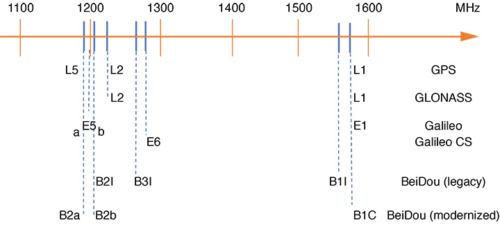
The modernization of GNSS includes satellites transmitting signals on multiple frequencies. The 12 GPS Block IIF satellites currently in orbit already broadcast the L5 signal, and all Galileo and BeiDou satellites launched so far have triple-frequency capabilities. In November 2017, the BeiDou constellation began a new phase of its development with the launch of the Beidou-3S satellites offering new signals compatible with the GPS L1/L5 bands. In March 2018, the European Union decided to open its Commercial Service (CS), offering at no cost the signal and correction stream for the “CS high accuracy” service. As a result, the E6 signal is now available on 14 satellites and can be tracked by modern GNSS receivers. FIGURE 1 depicts the frequency plan of the open GNSS signals, including these last evolutions, as of May 2018.
With three or more frequencies, a series of widelane ambiguities can be resolved in a cascading scheme. These unambiguous widelane signals can be used to form an ionosphere-free phase measurement with lower noise than code measurements, but typically still at the decimeter level. The availability of the Galileo E6 signal provides a significant step forward for PPP-AR, permitting instantaneous convergence. As a result of frequency separation, unambiguous widelane signals have low noise characteristics, which further benefits the resolution of the whole set of ambiguities. The strategy used in our study is a generalization of the widelaning technique, based on uncombined observations, which we describe as Optimal Estimation using Uncombined Four-frequency Signals (OEUFS).
We explain how instantaneous centimeter-level PPP is achieved by first analyzing the precision of the ambiguity and range parameters in the single-satellite case. The network estimation of the uncombined Galileo phase biases is then described, followed by epoch-by-epoch and 5-minute PPP solutions based on OEUFS.
SINGLE-SATELLITE PROCESSING
To get a first grasp of the benefits of using four frequencies, we first look into single-satellite data. The aim of this analysis is twofold: first, to evaluate the ability of fixing linear combinations of ambiguities and, second, to determine the resulting precision of the unbiased range estimate once these ambiguities are fixed.
Uncombined observations on four Galileo frequencies (E1, E5a, E5b and E6) are used to model an ionosphere-free range, a slant ionospheric delay, and four carrier-phase ambiguities. It should be noted that measurements on a fifth frequency (E5) are available but, due to the proximity of E5 with respect to E5a and E5b, its impact was found to be almost negligible. We will, therefore, restrict ourselves to the four-frequency case. Only two code observations are included in the model — in this case E1 and E5a — since adding other frequencies would require the estimation of differential code biases. Thus, for single-epoch processing, additional code measurements would not usefully contribute to the solution. Observable standard deviations are set to 3 millimeters and 30 centimeters for carrier phase and code, respectively. An analysis using a zero-length baseline revealed that weak correlations do exist between signals, and multipath effects could further increase this correlation. Although taking into consideration correlations among observations would lead to a more realistic covariance matrix, these correlations were neglected in producing the results shown in this article. This is justified by the fact that correlation coefficients are usually not available, especially for real-time processing.
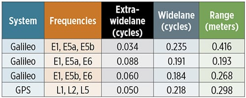
The above-mentioned model was inverted in a least-squares adjustment to perform covariance analysis. While the Least‐squares AMBiguity Decorrelation Adjustment (LAMBDA) method can be used for the identification of optimal linear combinations of ambiguities, the classic widelane ambiguities were found to perform equally well and were used in our work to simplify the exposition. When no ambiguities are fixed, the quality of the solution is driven by the noise on the code observations. TABLE 1 shows that, in this case, the receiver-satellite range parameter can be estimated with a precision of 0.776 meters. This value can be translated into a 3D-position precision by using the position dilution of precision (PDOP) factor. As a rule of thumb, if the PDOP for all satellites in view is equal to 1, the resulting 3D precision should be around 78 centimeters.
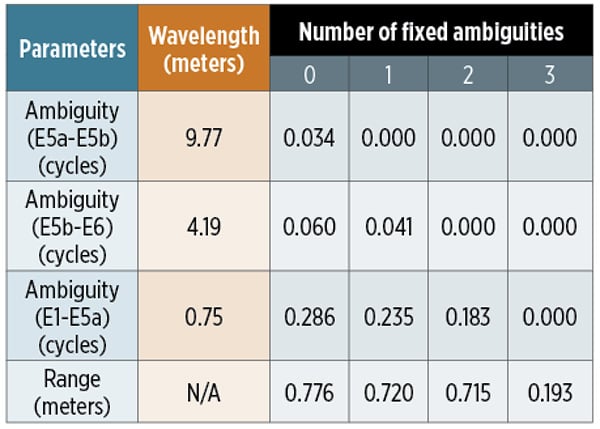
Even though the range is not very precise, forming the E5a-E5b widelane ambiguity from the estimated uncombined ambiguities gives a precision of 0.034 cycles, which can be reliably fixed due to the very long wavelength of the signal (9.77 meters). Adding this constraint to the system allows us to estimate the E5b-E6 widelane ambiguity with a standard deviation of 0.041 cycles (although it could also have been fixed initially). Interestingly, fixing both extra-widelane ambiguities does not significantly improve the precision of the range information derived from a single satellite. Nevertheless, due to correlations among ambiguity parameters, a precision of 0.183 cycles is now obtained for the E1-E5a widelane, an improvement of approximately 35 percent over the initial estimate.
While the E1-E5a ambiguity is not sufficiently precise for reliable instantaneous fixing based on single-satellite data from one epoch, using the geometric information from several satellites will enable single-epoch ambiguity resolution for three widelane ambiguities per satellite, as we show in the following sections. Assuming for the moment that ambiguity resolution was indeed successful on all three widelanes, Table 1 indicates that the range parameter can now be estimated with a standard deviation of 19 centimeters, a substantial improvement over the initial 78-centimeter precision. Recalling the PDOP factor introduced above, instantaneous 3D position precision at the 20-centimeter mark should then be possible with good geometry.
Including all available measurements in the model necessarily leads to the best performance. Still, TABLE 2 presents the conditional precision of parameters in three-frequency configurations. The precision for the widelane ambiguity is conditioned on first fixing the extra-widelane ambiguity, while that for the range assumes fixed extra-widelane and widelane ambiguities. The table highlights that frequency spacing plays a key role in the system performance. After fixing two widelane ambiguities, the Galileo E1-E5a-E5b configuration provides a range with a standard deviation of approximately 42 centimeters. The E1-E5a-E6 configuration is the best option, with a precision of the range parameter equal to the four-frequency case. In other words, the contribution of the E5b signal is almost negligible once the E5a-E6 ambiguity, having a wavelength of 2.93 meters, is resolved. For comparison purposes, the values for GPS are included and show that Galileo has the potential for significantly more precise instantaneous positioning.
NETWORK SOLUTION
To demonstrate the concept of four-frequency ambiguity resolution for PPP, a phase-bias network solution for the Galileo constellation must be generated. Our solution is based on the precise satellite orbit and clock corrections produced by the Centre National d’Études Spatiales (CNES) as a part of the International GNSS Service (IGS) Multi-GNSS Experiment (MGEX). These products contain satellite clock corrections at a 30-second interval, as well as widelane biases allowing for GPS ambiguity resolution in the L1 and L2 frequency bands. For this reason, the following analysis considers both GPS and Galileo constellations.
Consistent processing of multi-frequency and multi-modulation signals requires code-bias corrections. The differential code-bias products from the German Aerospace Center (DLR), including the Galileo E6 signals, are used. Ambiguity resolution for Galileo can only be enabled with corresponding phase biases for all frequencies. To this date, the main contributors to the IGS for E6-compatible receivers are Natural Resources Canada (NRCan), CNES and Geoscience Australia. Since a global network of ground receivers tracking all four Galileo frequencies is not yet available, our solution is computed from a regional, but wide-area, network in Australia. The network consists of six reference stations with multi-system, multi-frequency receivers as depicted with red triangles in FIGURE 2. (Station CEDU is not included in the network solution because it is used later as a rover for PPP testing.) Measurements collected at a 30-second interval are retrieved from the Crustal Dynamics Data Information System (CDDIS) data archive. For the purpose of our demonstration, data from April 1, 2018, from 13:45:00 to 14:35:00 GPS Time is selected. During this period, five Galileo satellites were continuously tracked by the Australian stations, allowing the computation of a Galileo-only solution.
The phase-bias solution is a generalization in the multi-frequency case of the well-known widelane/narrowlane GPS scheme. The first step consists of resolving all integer ambiguities in the network. As we deal with four frequencies, it is required to fix four ambiguities, or their combinations, per satellite-station pass. The first three combinations used for this study are the widelanes defined from E5a-E1, E5b-E1 and E6-E1. Their ambiguities are solved, as for the dual-frequency GPS case, thanks to the Melbourne-Wübbena combination. Then, one remaining integer ambiguity (here, E1) is solved by forming the ionosphere-free phase combination between E1 and E5a (with the corresponding widelane ambiguity already resolved as an integer value). The second step aims at recovering the uncombined phase biases from the estimated linear combinations of biases. By a simple system inversion, it is possible to reconstruct the phase biases on each frequency.
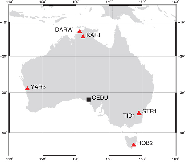
FIGURE 3 shows the estimated biases for each frequency over the study period. The values were shifted by an integer number of the carrier wavelength for plotting purposes. The uncombined biases obtained are relatively stable, although they vary by a few centimeters over this one-hour period. These fluctuations are correlated among frequencies due to the transformation from linear combinations to uncombined biases. It should be understood that the resulting biases are not true phase biases, but rather biases to be applied to the carrier-phase observations.

PRECISE POINT POSITIONING
We assessed the impact of using four frequencies transmitted by Galileo (E1, E5a, E5b and E6) on positioning performance by using station CEDU in Australia (see Figure 2). It is equipped with a multi-frequency receiver collecting multi-GNSS observations at 30-second intervals. Position estimates are derived from the PPP methodology using the satellite orbit and clock corrections, along with the carrier-phase and code biases, described in the previous section.
We computed three different solutions:
- a GPS-only solution;
- a Galileo-only solution; and
- a GPS and Galileo combined solution.
For all solutions, all error sources affecting observations are modeled, including relativistic and wind-up effects, solid Earth tides and ocean loading. The a priori tropospheric zenith delay (TZD) is computed using the Vienna Mapping Function 1 (VMF1) grids, while a priori ionospheric delays are obtained from a global ionospheric map (GIM) generated at the Center for Orbit Determination in Europe (CODE). The eccentricity between the satellite antenna phase centers and the satellite center of mass is obtained from the latest version of the IGS ANTEX file, which includes frequency-dependent phase-center offsets and variations for Galileo. Since there are no Galileo-specific ground-antenna calibrations available, GPS values are used as approximations.
In all cases, we processed uncombined observations corresponding to the OEUFS strategy. For GPS, the L1C and L2W carrier-phase observations are used, along with the C1W and C2W code observations. For Galileo, the L1C, L5Q, L6C and L7Q carrier phases are used, with identical modulations for code measurements. Note that this signal identification uses the RINEX 3 conventions where, for Galileo, the L5 and L7 signals correspond to those in the E5a and E5b bands, respectively. Carrier-phase observations are given a standard deviation of 2 millimeters at zenith, while code observations are deweighted by a factor of 100. An elevation-angle-dependent weighting strategy also assigns lesser weight to satellites closer to the local horizon. Therefore, the value of 3 millimeters used in the single-satellite analysis above corresponds to a satellite tracked at an elevation angle of approximately 40 degrees.
The PPP filter includes states for the three position components, one receiver clock parameter per satellite system, inter-frequency code biases, one phase-bias parameter per frequency, a residual TZD, a residual slant ionospheric delay per satellite and carrier-phase ambiguities. To confirm the theoretical analysis from a previous section, the empirical single-epoch ambiguity-fixing success rate is first evaluated using a bootstrapping algorithm. The full vector of estimated float ambiguities is first decorrelated using the LAMBDA method, and all ambiguities having a success rate larger than 99 percent are fixed to integers. FIGURE 4 shows the number of fixed ambiguities for each solution.
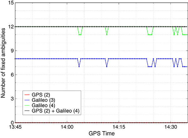
Not surprisingly, the dual-frequency GPS solution is incapable of reliably fixing ambiguities within a single epoch. During this time period, five Galileo satellites are tracked. If we first consider all four frequencies from Galileo, and use the ambiguities on one satellite to provide the datum, then a total of 16 ambiguities are being estimated in the PPP filter, 12 of which are considered widelanes. Figure 4 confirms that using correlations introduced by the geometry allows instantaneous fixing of all widelane ambiguities for Galileo for most epochs. Adding GPS to the Galileo solution makes Galileo widelane fixing more reliable, but does not allow fixing of additional ambiguities. The three-frequency (E1, E5a and E6) Galileo configuration also enables instantaneous fixing of all eight widelane ambiguities, since the inclusion of E5b brings minimal additional information.
In all subsequent solutions, ambiguity estimation is performed using a more sophisticated method referred to as the best integer equivariant (BIE) approach. Because it is expected that not all ambiguities can be fixed simultaneously, a partial ambiguity resolution scheme is required. The BIE method fulfills this criterion by computing a weighted average of integer vectors. The outcome is a constrained ambiguity vector whose entries take either integer or float values. The key point of this approach is that the BIE float estimates can be improved by the averaging process with respect to the least-squares float estimates. Furthermore, by exploiting the correlations contained in the ambiguity covariance matrix, this method can effectively fix linear combinations of ambiguities. Therefore, we are not explicitly forming widelane ambiguities, but rather optimal linear combinations of ambiguities are fixed through the BIE averaging process. This strategy is implemented using the LAMBDA method to decorrelate ambiguities. Even though the BIE estimates are independent of the decorrelation, this step improves the computational efficiency of the approach.
As we explained in the previous sections, positioning with fixed widelane ambiguities can potentially allow for instantaneous precise positioning. FIGURE 5 demonstrates the epoch-by-epoch position estimates for the three solutions. As the strategy implies, the filter is entirely reset between epochs, and each point in the time series is independently determined. As expected, instantaneous ambiguity resolution with GPS alone is not feasible. Although the external information provided by the GIM is beneficial in reducing the errors, the root-mean-square (RMS) error is at the decimeter level for all components (see TABLE 3).

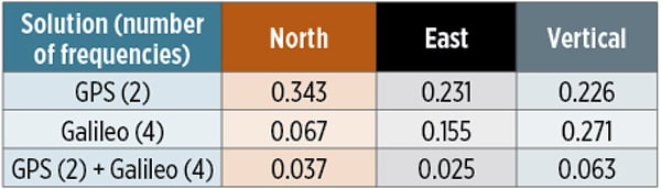
The Galileo-only solution offers a substantial improvement in the horizontal components. These results are explained by the ambiguity-resolved widelane signals providing precise range estimates. It should be noted that only five Galileo satellites are visible during this period with a PDOP slightly exceeding a value of 3. When the full constellation of satellites will be in orbit, even better results could be obtained from a Galileo-only solution. The three-frequency (E1, E5a, E6) Galileo solution offers almost identical position estimates and is not shown here for conciseness. Combining GPS and Galileo yields the best solution with centimeter-level instantaneous positioning (refer to Table 3). For several epochs, a fully converged position is even obtained within a single epoch.
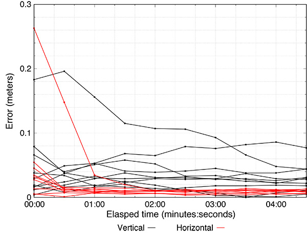
While the RMS errors of the combined GPS + Galileo solution is at the centimeter level, individual epochs can still exhibit decimeter-level errors. To demonstrate the convergence capabilities of the OEUFS strategy, we computed 5-minute PPP sessions. Even though the station is stationary, we added a large amount of process noise to the position states to simulate kinematic processing. FIGURE 6 shows the results of all 10 sessions: horizontal convergence to a few centimeters could be achieved within two epochs in all but one session.
CONCLUSION
We have shown that GNSS modernization is a key component for reducing the convergence time of PPP solutions. Combining multiple constellations strengthens the geometry, and using multiple frequencies allows for improved ambiguity resolution performance. In particular, tracking of the E6 Galileo commercial service signal turns out to be particularly beneficial in terms of instantaneous positioning capabilities. We demonstrated that ambiguities can be instantaneously resolved on Galileo satellites, leading to a range estimate approximately four times better than that provided using code measurements. With good satellite geometry, these frequencies can enable instantaneous 3D positioning with an accuracy of around 20 centimeters. Combining Galileo and GPS allows for single-epoch centimeter-level PPP solutions and full convergence within a few epochs.
We expect that the robustness and accuracy of the OEUFS strategy will improve in the future, with an increasing number of multi-frequency satellites and ground stations. Specifically, the additional frequencies provided by BeiDou and the Quasi-Zenith Satellite System will enhance the geometry of the solution and will further expedite convergence. Within a few years, instantaneous PPP might very well become a practical alternative to RTK for a wide range of applications.
ACKNOWLEDGMENTS
The authors acknowledge Geoscience Australia for making publicly available modernized GNSS data, as well as Paul Collins from NRCan for the review of our manuscript and technical advice. This article is published as NRCan Contribution 20180102.
MANUFACTURER
All of the stations used for the tests described in this article have PolaRx5 reference receivers manufactured by Septentrio (www.septentrio.com).
DENIS LAURICHESSE is a member of the Navigation Systems Department at CNES in Toulouse, France. He has been in charge of the DIOGENE GPS orbital navigation filter, and is now involved in navigation algorithms for GNSS. He is in charge of the CNES IGS real-time analysis center. Laurichesse was the co-recipient of the 2009 Institute of Navigation Burka Award for his work on phase ambiguity resolution.
SIMON BANVILLE is a senior geodetic engineer with the Canadian Geodetic Survey of NRCan, Ottawa, Canada, working on PPP. He obtained his Ph.D. degree in 2014 from the Department of Geodesy and Geomatics Engineering at the University of New Brunswick, under the supervision of Richard B. Langley. He is the recipient of the Institute of Navigation 2014 Parkinson Award.
FURTHER READING
• Precise Point Positioning
“Where Are We Now, and Where Are We Going?: Examining Precise Point Positioning Now and in the Future” by S. Bisnath, J. Aggrey, G. Seepersad and M. Gill in GPS World, Vol. 29, No. 3, March 2018, pp. 41–48.
“Precise Point Positioning” by J. Kouba, F. Lahaye and P. Tétreault, Chapter 25 in Springer Handbook of Global Navigation Satellite Systems, edited by P.J.G. Teunissen and O. Montenbruck, published by Springer International Publishing AG, Cham, Switzerland, 2017.
• Multi-GNSS Experiment
“The Multi-GNSS Experiment (MGEX) of the International GNSS Service (IGS) – Achievements, Prospects and Challenges” by O. Montenbruck, P. Steigenberger, L. Prange, Z. Deng, Q. Zhao, F. Perosanz, I. Romero, C. Noll, A. Stürze, G. Weber, R. Schmid, K. MacLeod and S. Schaer in Advances in Space Research, Vol. 59, No. 7, April 2017, pp. 1671–1697, doi: 10.1016/j.asr.2017.01.011.
“Getting a Grip on Multi-GNSS: The International GNSS Service MGEX Campaign” by O. Montenbruck, C. Rizos, R. Weber, G. Weber, R. Neilan and U. Hugentobler in GPS World, Vol. 24, No. 7, July 2013, pp. 44–49.
• PPP Carrier-Phase Ambiguity Resolution and Convergence
“Carrier-phase Ambiguity Resolution: Handling the Biases for Improved Triple-frequency PPP Convergence” by D. Laurichesse in GPS World, Vol. 26, No. 4, April 2015, pp. 49-54.
“Zero-difference GPS Ambiguity Resolution at CNES–CLS IGS Analysis Center by S. Loyer, F. Perosanz, F. Mercier, H. Capdeville, and J.C. Marty in Journal of Geodesy, Vol. 86, No. 11, Nov. 2012, pp. 991–1003, doi: 10.1007/s00190-012-0559-2.
“Undifferenced GPS Ambiguity Resolution Using the Decoupled Clock Model and Ambiguity Datum Fixing” by P. Collins, S. Bisnath, F. Lahaye and P. Héroux in Navigation, Vol. 57, No. 2, Summer 2010, pp. 123–135, doi: 10.1002/j.2161-4296.2010.tb01772.x.
• Least‐squares AMBiguity Decorrelation Adjustment (LAMBDA)
“Carrier Phase Integer Ambiguity Resolution” by P.J.G. Teunissen, Chapter 23 in Springer Handbook of Global Navigation Satellite Systems, edited by P.J.G. Teunissen and O. Montenbruck, published by Springer International Publishing AG, Cham, Switzerland, 2017.
“Theory of Integer Equivariant Estimation with Application to GNSS” by P.J.G. Teunissen in Journal of Geodesy, Vol. 77, No. 7-8, Oct. 2003, pp. 402–410, doi: 10.1007/s00190-003-0344-3.
“A New Way to Fix Carrier-phase Ambiguities” by P.J.G. Teunissen, P.J. de Jonge, and C.C.J.M. Tiberius in GPS World, Vol. 6, No. 4, April 1995, pp. 58–61.