No audio available for this content.
The military is always looking at new techniques and technology for deriving position and, it seems, every few years signals of opportunity (SOOP) becomes fashionable again.
In broad terms, SOOP refers to the use of any signals for navigation, which are not normally intended for navigation. This might mean TV or radio broadcast signals, cellular network signals, or anything else you can receive.
The promise of SOOP
In the quest for resilient positioning and navigation, SOOP certainly sounds attractive. When GPS goes down, why not simply continue to navigate by receiving digital TV signals instead? Why not receive a whole pile of different signals, and make yourself virtually immune to jamming?
You can even turn jamming from a problem to a solution. If someone does decide to turn on a bunch of jammers, why not use the jammers themselves as signals of opportunity, and position yourself using those? With so many possibilities, it’s no wonder SOOP excites people. Certainly it’s of great interest to the military of many countries.
Let’s dip our toes into the world of opportunistic navigation.
What signals might we use?
The figure below shows what we get if you use a spectrum analyzer to quickly sample what’s on the airwaves in the UK, in this case looking fairly coarsely from 10 MHz to 3 GHz. A number of candidate signals immediately present themselves, which are labeled 1 to 11 and identified in the table.
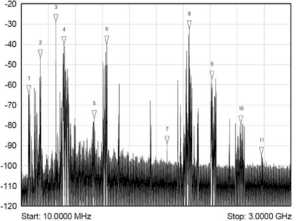
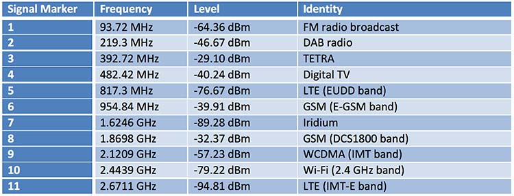
There are, of course, many more signals-of-opportunity out there, but this illustrates a few of the more visible ones. How do we go about using these signals for positioning ourselves?
Bringing in defense techniques
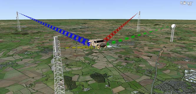
For decades, one of the principle requirements in electronic warfare (EW) has been to geolocate enemy transmissions. This has given rise to a plethora of techniques for determining location, such as received signal strength (RSS), angle-of-arrival (AOA), time-of-arrival (TOA), time difference of arrival (TDOA), frequency difference of arrival (FDOA), and so on.
In a positioning application, we have the reciprocal problem: instead of trying to geolocate a transmitter relative to ourselves, we are trying to geolocate ourselves relative to a set of transmitters. But of course we use the same techniques: GPS is an excellent example of a TOA system.
Let’s look at the basics of TDOA. A signal s arriving at location 1 can be expressed as
![]()
where A1 is an amplitude scaling to account for attenuation over the path, n1 is additional noise, and d1 is the signal delay time. We can repeat the equation for further locations:
![]()
Usually we designate one location as the reference, in which case we can rewrite the above equations as:
![]()
![]()
The first problem is to determine D, the time difference of arrival. There are many ways to do this, but a popular method is to perform generalized cross-correlation:
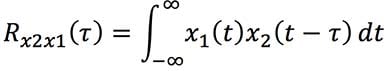
Or, in a realizable digital form:
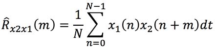
Finding the peak of this function gives us our estimate of the time difference D. It’s a little bit more involved in practice, as we would normally apply filtering functions to improve the TDOA resolution, but you get the idea. Each TDOA measurement gives a set of possible locations that form a hyperboloid. With three stations, we will have two hyperboloids, the intersection of which gives a set of possible locations along a hyperbola. The addition of a fourth signal allows us to plot three hyperboloids, from which we can then determine position.

There are various ways to solve for the hyperbolic intersections. With only four measurements it is possible to compute the solution analytically, but with many measurements an iterative approach or minimum mean squared error technique is often used.
TDOA, when used properly, can form the basis of a highly accurate positioning system. A number of navigation systems utilize TDOA technology, such as LORAN and its variants.
Now let’s consider angle-of-arrival. AOA techniques generally make use of an antenna array to provide spatial diversity, allowing the direction of a source transmission to be determined. Measured angles to multiple transmitters then allows triangulation to be performed and the position computed. There are some advantages to AOA techniques, when compared to TDOA: position can be computed with as few as three signals, there is no requirement for time synchronization in any form, and narrowband signals can be used without loss of accuracy. Disadvantages include larger physical size due to the use of an array of antennas, and potentially more susceptible to environmental effects such as multipath.
Classical AOA methods include Capon’s method, but since the 1980s the preferred techniques have often been signal subspace methods such as Multiple Signal Classification (MUSIC), Estimation of Signal Parameters by Rotational Invariance Techniques (ESPRIT), and variants of these techniques. The most well known of the subspace methods, MUSIC, performs an eigendecomposition of the sample covariance matrix given by:
![]()
Once the signal and noise eigenvectors have been separated the array manifold is projected into the appropriate subspace to yield the MUSIC surface:
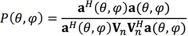
The peaks of the function P, give us the direction-of-arrival of any signals. From these multiple lines of bearing we can perform triangulation, and derive our position.
We’ve looked at TDOA and AOA methods, which are just two of many techniques that can be used to process signals-of-opportunity to derive position. But there are some perceived drawbacks to navigation by SOOP. By definition, SOOP makes use of transmitters that are uncooperative, and not generally designed with navigation in mind.
For TDOA you are dependent on signals that are transmitted synchronously (or else you need a separate source of reference), which may or may not be the case. You also need to know the locations of the various transmitters, for example the coordinates of any GSM base stations, digital TV transmitters, and so on. It may be difficult to obtain this information, especially in some parts of the world. But whilst it certainly helps to have this information, it isn’t entirely necessary. It is possible to both position yourself, and build up a map of the transmitter locations, without a-priori information.
SLAM
Simultaneous localization and mapping (SLAM) is a field popular in the autonomous vehicle and robotics communities. It’s often described as a machine-learning concept, which aims to solve the problem of positioning oneself within a map, whilst simultaneously constructing and updating that map. There are a pile of techniques and algorithms that have been applied to the problem, including the good old Kalman filter, and the particle filter.
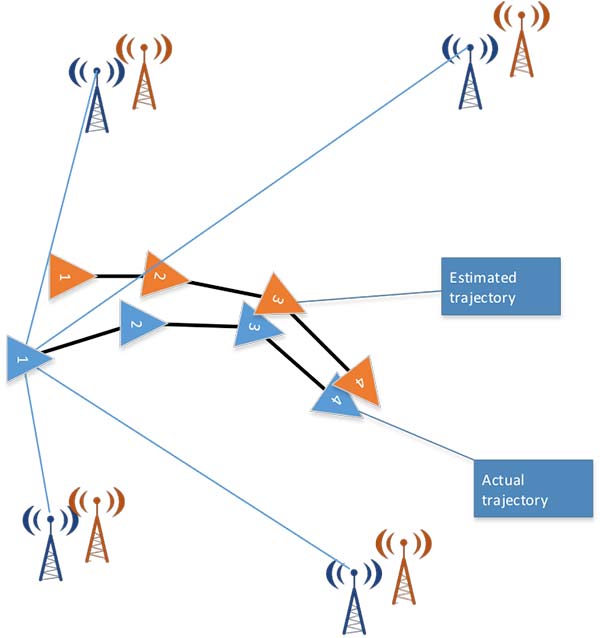
In basic SLAM, you use a state vector to store an estimate of your position (and often orientation as well), just as you would in a typical GPS receiver. However, in SLAM, we also store estimates of the transmitter positions (called “features” in SLAM terminology). If we want to localize ourselves in a global coordinate frame it does mean we need an initial estimate of our position from some other means, like GPS. Otherwise we can only localize ourselves within the map we are generating.
From our initial position estimate, we then move in some way. We then estimate our position again, perhaps using some form of dead reckoning technique, like inertial or visual odometry. Together with our motion model, this forms the prediction phase of the Kalman filter. We perform the measurement phase by re-measuring any features (our transmitters of opportunity), along with any new ones.
If you know about Kalman filters, you might spot one of the problems with SLAM: As the number of features increases, the size of the state vector becomes larger, until you end up with huge matrices that are very time-consuming to solve. The solution time is a quadratic function of the number of state variables. For this reason, it is often necessary to constrain the problem in some way: perhaps by limiting the number of transmitters we keep track of.
But when done properly, SLAM is a powerful technique for signals-of-opportunity navigation.
Is SOOP worth it?
We’ve seen that, by using a variety of techniques, almost any radio signal can be used for opportunistic navigation purposes.
One disadvantage of SOOP is that it can require complex hardware to do it well. If you truly want to use all the opportunistic signals out there, then you need a receiver that can handle a very wide range of frequencies. You also need an antenna or set of antennas that can do the same.
When resilient PNT is a critical military requirement, you cannot afford to rely on signals that you don’t control. SOOP is also highly dependent on where you are. There aren’t many opportunistic signals at sea or in the desert, compared to in the urban environment (perhaps the odd satellite signal, or HF signal).
So SOOP is unlikely to become a primary technology for the military. But it does have the potential to be a powerful augmentation to GNSS, and it certainly deserves a place in the PNT kit bag.
Figures: Michael Jones