Toward a Unified PNT — Part 2

Photo: peeterv/iStock/Getty Images Plus/Getty Images

Ambiguity and Environmental Data: Two Further Key Challenges of Multisensor Positioning

By Paul D. Groves, Lei Wang, Debbie Walter, and Ziyi Jiang, University College London

The coming requirements of greater accuracy and reliability in a range of challenging environments for a multitude of mission-critical applications require a multisensor approach and an over-arching methodology that does not yet exist. Part 1 of this article, in the October issue, examined the two key concepts of complexity and context. In this continuation, we complete our overview with exploration of the requirements of ambiguity and environmental data.

Ambiguity occurs when measurements can be interpreted in more than one way, leading to different navigation solutions, only one of which is correct. Any navigation technique can potentially produce ambiguous measurements. The likelihood depends on both the positioning method and the context, both environmental and behavioral. Urban and indoor positioning techniques that do not require dedicated infrastructure are particularly vulnerable to ambiguity. Poor handling of ambiguity results in erroneous navigation solutions and the navigation system can become “lost,” whereby it is unable to recover and may even reject correct measurements.

There are six main causes of ambiguity: feature identification, pattern matching, propagation anomalies, geometry, system reliability, and context ambiguity. Each of these is described in turn below.

Feature Identification Ambiguity. The proximity, ranging, angular positioning, and Doppler positioning methods all use landmarks for positioning. These may be radio, acoustic, or optical signals, or natural or man-made features of the environment. For reliable positioning, these signals or features must be correctly identified.

Digital signals intended for positioning incorporate identification codes. However, where a signal is weak and/or interference is high, it may be possible to use the signal for positioning but not decode the identification information. For signals of opportunity — that is, not designed for positioning — the identification codes may be encrypted, while analog signals do not typically have identifiers. These signals must be identified using their frequencies and an approximate user position, in which case there may be multiple candidates. Even where a signal of opportunity is identifiable, the transmission site may change without warning. For example, Wi-Fi access points are sometimes moved and mobile phone networks are periodically refigured. Thus, there is a risk of false landmark identification.

Environmental features are difficult to identify uniquely. In image-based navigation, man-made features, such as roads, buildings, and signs, are easiest to identify in images due to their line and corner features. However, similar objects are often repeated in relatively close proximity. For example, Figure 18 shows the locations of the five “no entry” signs in a 1,200-meter circuit of Central London streets. Two of the signs are within 20 meters of each other. (Figure numbering continues the sequence beginning in Part 1, October issue.)

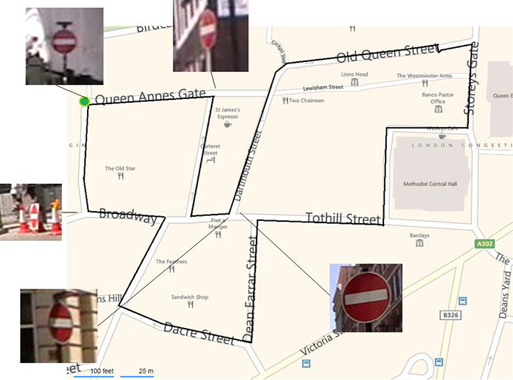
Figure 18. “No entry” signs in a 1,200-meter circuit of Central London. (Background image courtesy of Bing maps | Photo: Paul D. Groves, Lei Wang, Debbie Walter and Ziyi Jiang, University College London)

Pattern-Matching Ambiguity. The pattern-matching positioning method maintains a database of measurable parameters that vary with position. Examples include terrain height, magnetic field variations, Wi-Fi signal strengths, and GNSS signal availability information. Values measured at the current unknown user position are compared with predictions from the database over a series of candidate positions. The position solution is then obtained from the highest scoring candidate(s).

An inherent characteristic of pattern matching is that there is sometimes a good match between measurements and predictions at more than one candidate position. Figure 19 and Figure 20 show GNSS shadow-matching scoring maps based on smartphone measurements taken at the same location 40 seconds apart. The scores are obtained by comparing GNSS signal-to-noise measurements with signal availability predictions derived from a 3D city model. In Figure 19, maximum scores (shown in dark red) are only obtained in the correct street, whereas in Figure 20, there is also a high-scoring area in the adjacent street, giving two possible position solutions.

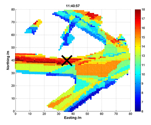
Figure 19. GNSS shadow-matching scoring map – unambiguous case (the cross shows the true position and white areas are indoor locations). (Photo: Paul D. Groves, Lei Wang, Debbie Walter and Ziyi Jiang, University College London)

Figure 20. GNSS shadow-matching scoring map – unambiguous case (the cross shows the true position and white areas are indoor locations). (Photo: Paul D. Groves, Lei Wang, Debbie Walter and Ziyi Jiang, University College London)

Figure 21 presents another example, showing the height of a road vehicle derived from a barometric altimeter at three different times. Provided the altimeter is regularly calibrated, it may be used for terrain-referenced navigation (TRN), determining the car’s position along the road by comparing the measured height with a database. However, if only the current height is compared, it will typically match the database at multiple locations within the search area, as the figure shows. The ambiguity can be reduced by comparing a series of measurements from successive epochs, known as a transect, with the database. This approach is applicable to any pattern-matching technique. However, increasing the transect length to reduce the ambiguity also reduces the update rate, and the ambiguity problem can never be eliminated completely.

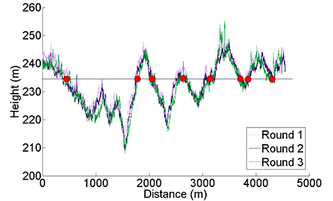
Figure 21. Height of a car derived from a barometric altimeter at three different times; readings of around 235 m are highlighted. (Photo: Paul D. Groves, Lei Wang, Debbie Walter and Ziyi Jiang, University College London)

Signal Propagation Anomalies. The ranging, angular positioning, and Doppler positioning methods all make the assumption that the signal propagates from the transmitter (or other landmark) to the user in a straight line at constant speed. Significant position errors can therefore arise when these assumptions are not valid due to phenomena such as non-line-of-sight reception, multipath interference, and severe atmospheric refraction. In challenging environments, such as dense urban areas and indoors, multiple signals are typically affected by propagation anomalies, and it is not always easy to determine which signals are contaminated.

Where the position solution is overdetermined (that is, more than the minimum number of signals are received), different combinations of signals will produce different position solutions when there are significant propagation anomalies. 

Figures 22 and 23 illustrate this for conventional GNSS positioning using a Leica Viva geodetic receiver, showing the position errors obtained using different combinations of GPS and GLONASS signals. In Figure 22, the receiver is located on a high rooftop and the majority of position solutions are within 15 meters of the mean, with the remainder easily dismissible as outliers. However, in Figure 23, where the receiver is located in a dense urban location, the candidate position solutions are spread over more than 100 meters, and the correct position solution is not clear. The densest cluster of positions is far from both the centroid and the truth. Therefore, anomalous signal propagation may be treated as an ambiguity problem.

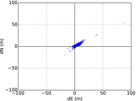
Figure 22. GNSS position errors using different combinations of signals in a rooftop environment. (Photo: Paul D. Groves, Lei Wang, Debbie Walter and Ziyi Jiang, University College London)

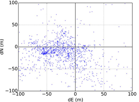
Figure 23. GNSS position errors using different combinations of signals in a dense urban environment. (Photo: Paul D. Groves, Lei Wang, Debbie Walter and Ziyi Jiang, University College London)

Geometric Ambiguity. Geometric ambiguity occurs when more than one position solution may be derived from a set of otherwise unambiguous measurements. Figure 24 shows two examples. On the left, two ranging measurements in two dimensions produce circular lines of position that intersect in two places. On the right, a ranging measurement and a direction-finding measurement are made using the same signal. As direction finding has a 180° ambiguity, the lines of position also intersect at two places.

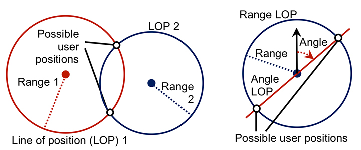
Figure 24. Geometric ambiguity in two dimensions from two ranging measurements (left), and a ranging and direction-finding measurement (right). (Photo: Paul D. Groves, Lei Wang, Debbie Walter and Ziyi Jiang, University College London)

System Reliability. Navigation subsystems can produce incorrect information for a host of different reasons. Some examples include:

• user equipment hardware and software faults;
• transmitter hardware and software faults;
• out-of-date databases used for pattern matching, including TRN, GNSS shadow matching, and map matching;
• wheel slips in odometry;
• the effects of passing vehicles and animals on environmental feature visibility, availability and strength of radio signals, and Doppler-based dead reckoning.

Some of these failure modes are easily detectable through the measurements failing basic range checks or being absent altogether. In other cases, faults may be detected by consistency checks within the subsystem. For example, wheel slip may be detected by comparing measurements from different wheels, while Doppler radar and sonar systems typically incorporate a redundant beam to enable the interruption of a beam by a vehicle or animal to be detected.

Subsystems can sometimes output incorrect information that is plausible. An ambiguity thus exists where it is uncertain whether or not a measurement may be trusted. An ambiguity also exists where a fault has been detected, but not its source. Thus, some of the information produced by the subsystem must be incorrect, but some of it may be correct.

Context Ambiguity. As discussed in Part 1 of this article (October issue), the optimum way of processing sensor information depends on the context. However, if context information is used, the navigation solution will then depend on the assumed context. For example, if an indoor environment is assumed, indoor radio positioning and map-matching algorithms that are only capable of producing an indoor position solution may be used. Similarly, if an urban environment is assumed, GNSS shadow matching and outdoor map matching may be selected, resulting in an outdoor position solution. Adoption of pedestrian and vehicle motion constraints can also lead to different navigation solutions.

Context determination is not a completely reliable process. Therefore, to minimize the impact of incorrect context assumptions on the navigation solution, the context should be treated as ambiguous whenever there is significant uncertainty.

Possible Solutions

There is no obvious solution to the ambiguity problem. Instead, different approaches to integrating ambiguous information may be adopted depending on the relative priorities of solution availability, reliability, and processing load. The main approaches, illustrated in Figure 25, are discussed below. They all require the subsystems to present the different measurement hypotheses and their associated probabilities to the integration algorithm.

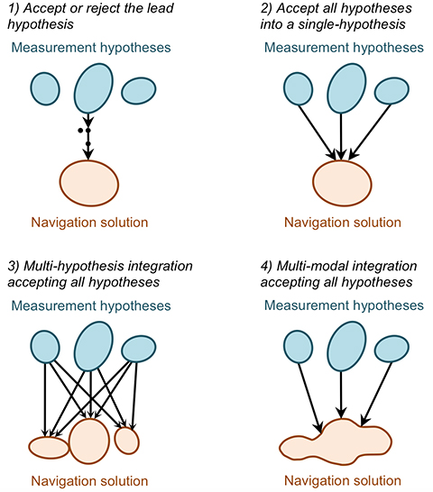
Figure 25. Methods of handling ambiguous measurements in a navigation integration algorithm. (Photo: Paul D. Groves, Lei Wang, Debbie Walter and Ziyi Jiang, University College London)

Accept or reject the lead hypothesis. The simplest way of handling ambiguous information is to maintain a single-hypothesis navigation solution and consider only the most-probable hypothesis from each subsystem. This is then accepted or rejected based on the following criteria:

• Whether the probability of the highest scoring hypothesis above a certain threshold.
• Whether the probability of the second-highest scoring hypothesis below a certain threshold.
• Whether the highest-scoring measurement hypothesis is consistent with the current integrated navigation solution. (Determinable using measurement innovation filtering.)

Context may be incorporated into this approach by accepting the highest-scoring behavioral and environmental contexts where they meet the above criteria and computing a context-independent navigation solution otherwise.

This approach is processor-efficient, but high integrity and availability cannot be achieved simultaneously. Low acceptance thresholds provide high reliability by rejecting most erroneous measurements, but low solution availability as many good measurements are also rejected. Conversely, high acceptance thresholds provide availability at the expense of reliability.

Accept all hypotheses into a single-hypothesis solution. A probabilistic data association filter (PDAF) accepts multiple measurement or context hypotheses, weighting them according to their probabilities, but represents the navigation solution as the mean and covariance of a uni-modal distribution. The measurement update to the state estimation error covariance matrix accounts for the spread in the hypotheses such that the state uncertainties can sometimes increase following a measurement update.

This approach reconciles the demands of integrity and availability at the price of a moderate increase in processing load. However, the uni-modal navigation solution can sometimes be misleading. For example, if a pattern-matching system determines that the user is equally likely to be in one of two parallel streets, the overall position solution will be midway between those streets.

Multi-hypothesis integration accepting all hypotheses. Multi-hypothesis integration deals with multiple measurement and context hypotheses by spawning multiple integration filters, one for each hypothesis. Each filter is allocated a probability based not only on the probabilities of the measurements input to it, but also on the consistency of those measurements with the prior estimates of that filter. This consistency-based scoring is essential; otherwise the filter hypothesis that inputs the highest-scoring measurement hypotheses will always dominate, regardless of whether those measurements are consistent across subsystems and successive epochs.

A fundamental characteristic of multi-hypothesis filtering is that the number of hypotheses grows exponentially from epoch to epoch. This is clearly impractical, so the number of hypotheses is limited by merging the lowest scoring hypotheses into higher scoring neighbors.

The overall navigation solution is the weighted sum of the constituent filter hypotheses. Each individual filter hypothesis describes a uni-modal distribution. However, the combined navigation solution is multi-modal. Thus, the position probability can be higher in two streets than in the buildings between those streets. This is a clear advantage over the PDAF-based approach, but the processing load is higher.

Multi-modal integration accepting all hypotheses. A multi-modal filter is not constrained to model the states it estimates in terms of a mean and covariance. This enables it to process multiple measurement and/or context hypotheses and represent the result as a weighted sum of the probability distributions arising from the individual hypotheses. Suitable data-fusion algorithms include the Gaussian mixture filter and the particle filter. A key advantage over multi-hypothesis integration is that measurements may be treated as continuous probability distributions instead of as a set of discrete hypotheses. This enables pattern-matching measurements to be integrated more naturally and offers greater flexibility in handling signal propagation anomalies.

A Gaussian mixture filter models the probability distribution of the navigation solution as the weighted sum of a series of multi-variate Gaussian distributions. An example is the iterative Gaussian mixture approximation of the posterior (IGMAP) technique, which has been applied to terrain referenced navigation integrated with inertial navigation.

A particle filter models the probability distribution of the navigation solution using a series of semi-randomly distributed samples, known as particles. Between a thousand and a million particles are typically deployed, with a higher density of particles in higher probability regions of the distribution. Particle filters have been used with a number of different navigation technologies, including TRN, pedestrian map matching, Wi-Fi positioning, and GNSS shadow matching.

Multi-modal integration algorithms offer the greatest flexibility in reconciling the demands of solution availability and reliability, but also potentially impose the highest processing load.

Issues to Resolve

The key challenge in handling ambiguous measurements is determining realistic probabilities for each hypothesis. A probability must also be calculated for the null hypothesis, that is, the hypothesis that every candidate measurement output by the subsystem is wrong. The same applies to ambiguous context.

A feature identification algorithm must allocate a score to every database feature that it compares with the sensor measurements. In practice, only features within a predefined search area, based on the prior position solution and its uncertainty, will be considered. Features scoring above a certain threshold will be possible matches. Similarly, pattern- matching algorithms allocate a score to each candidate position in the search area according to how well the sensor measurements match the database at that point. For correct handling of ambiguous matches, these scores should be as close as possible to the probabilities of the feature match or candidate position being correct.

Feature identification and pattern-matching algorithms can also fail to consider the correct feature or candidate position for several reasons. The correct feature or position may be outside the database search area. It may be absent due to the database being out of date. The sensor may also observe or be affected by a temporary feature that is not in the database, such as a vehicle. The null hypothesis probability must account for all of these possibilities. In practice, it will be higher where there is no good match between the measurements and database.

Signal propagation anomalies affect the error distributions of ranging, angle, and Doppler shift measurements, and the positions and velocities derived from them. These error distributions depend on whether the signals are direct line-of-sight (LOS), non-line-of-sight (NLOS), or multipath- contaminated LOS. However, this is not typically known. Signal strength measurements, environmental context, signal elevation (for GNSS), distance from the transmitter (for terrestrial signals), consistency between different measurements, and 3D city models can all contribute useful information. However, their relationship with the measurement errors is complex, so a semi-empirical approach is needed.

Moving on to reliability, virtually any subsystem can produce false information. The overall probability will typically be very low and thus only significant for high-integrity applications. However, the failure probability will be higher in certain circumstances, in which case the relevant subsystem should report a higher null probability. For example, in odometry, the probability of a wheel slip depends on host vehicle dynamics. Similarly, a radio signal is more likely to be faulty if it is weaker than normal. Repeated measurements, changes to the update interval, and sudden changes in a sensor output are also indicative of potential faults.

Geometric ambiguity is easy to quantify as the candidate solutions have equal probability in the absence of additional information.

As proposed in Part 1, the context determination process should produce multiple context hypotheses, each with an associated probability. Therefore, it is important to ensure that all navigation subsystems that use this context information do so in a probabilistic manner. Thus, where different context hypotheses lead to different values of the measurements output by a navigation subsystem, each measurement hypotheses should be accompanied by a probability derived from the context probabilities.

A further issue to resolve is the relationship between discrete and continuous ambiguity. Ambiguities in feature identification, solution geometry, failures, and context categorization are discrete and are suited to integration filters that treat them as a set of discrete hypotheses. However, the position solution ambiguity in pattern-matching is continuous, that is, the probability density is a continuous function of position, albeit sampled at discrete grid points. This probability distribution may be input directly to a particle filter. However, if the integration algorithm is a uni-modal filter or a bank of uni-modal filters, the probability distribution must be converted to a set of discrete hypotheses. This can be done by fitting a set of Gaussian distributions to the probability distribution. For signal propagation anomalies, their presence or absence is discrete. However, the resulting measurement error distribution is continuous, so a similar approach is appropriate.

The same challenging environments that require multiple navigation subsystems to maximize solution availability, accuracy, and reliability can also induce those subsystems to produce ambiguous measurements. Consequently, the modular integration architecture proposed in Part 1 should be capable of handling ambiguous measurements.

This is discussed further in our IEEE/ION PLANS 2014 paper, “The Four Key Challenges of Advanced Multisensor Navigation and Positioning.”

Environmental Data

Position-fixing systems need information about the environment, sometimes known as a “world model,” to operate. Proximity, ranging, and angular positioning all use landmarks that must be identified. For GNSS and other long-range radio systems, identification codes are determined when the system is designed and incorporated in the user equipment. However, this is not practical for shorter range signals, whether opportunistic or designed for positioning, due to the vast numbers of transmitters available worldwide and the fact that many will be installed during the lifetime of the user equipment. The user equipment will also require information on the characteristics of a signal to enable it to use that signal for ranging. A mobile device equipped with a generic radio or transceiver may be required to download software to enable it to use a proprietary indoor positioning system. For environmental feature-matching techniques, the user equipment requires information to enable it to identify each landmark.

Navigation using landmarks also requires their positions and, for passive ranging, their timing offsets. Signals designed for positioning typically provide this information, but it can take a long time to download (30 seconds for GPS C/A code) and can be difficult to demodulate under poor reception conditions. The positions of opportunistic radio transmitters and environmental features must be determined by other means.

For positioning using the pattern-matching method, a measurement of radio signal strength or a characteristic of the environment, such as the terrain height or magnetic field, is compared with a database to determine position. Therefore, a database providing values of the measured parameter over a regular grid of positions is required. Map matching requires a map database to indicate where the user can and cannot go. GNSS shadow matching requires a 3D city model to predict signal visibility.

Finally, as discussed in Part 1 of this article, mapping is required to determine environmental context information from the position solution and to enable location-dependent context connectivity information (for example, the location of train stations) to be used for context determination.

Possible Solutions

We discuss in turn the environmental data collection and its distribution to the user equipment.

Data Collection. Positioning data may be collected either from a systematic survey or by the users. In either case, regular updates will be required. A systematic survey might be conducted by the subsystem supplier, a national mapping agency, or a private third party. The user will need to pay for the data in some way. It could be included in the equipment cost, via a subscription payment, by accepting advertising, or through general taxation (for some national mapping agency data). For mobile devices, such as smartphones, mapping data may be available for some applications, but not others.

Single-user data collection does not involve user charges, but only provides data for places the user has already visited. A simple approach requires a good position solution to collect mapping data. This can work for applications that normally use GNSS, but require backups for temporary outages. However, it does not work for areas where GNSS reception is poor. Simultaneous localization and mapping (SLAM) techniques can perform mapping without a continuous position solution. However, there are several constraints. First, a good position solution that is independent of the data being mapped is required at some point, usually the start. Second, a navigation system including dead-reckoning technology must be used. Third, locations must be visited repeatedly within a short period of time (to achieve “loop closure”). Finally, only features close to the user can be mapped.

Cooperative mapping by a group of users solves many of the problems of single-user mapping. It can provide individual users with data for places they have not visited before. Distant landmarks can also be mapped more easily by multiple users, particularly where it is necessary to determine a timing offset as well as the location. However, a method for comparing and combining data from multiple users is required.

Data Distribution. For data collected by a systematic survey, there are two main data distribution models: pre-loading and streaming. Pre-loading requires sufficient user equipment data storage to cover the area of operation. New data may have to be loaded prior to a change in operating area, and updates will be required. However, a continuous communications link is not needed.

Streaming requires much less data to be stored by the user and provides up-to-date information, but only where a communications link is available. Although buffering can bridge short outages, navigation data is simply not available for areas without sufficient communications coverage. Continuous streaming can also be expensive. One solution is a cooperative approach using peer-to-peer communications for much of the data distribution. A pair of users traveling in opposite directions along the same route will each have data that is useful to the other. A further possibility is to incorporate local information servers in Wi-Fi access points for exchanging information relevant to the immediate locality. This might be best suited to indoor navigation, where there is an incentive for the building operator to provide the service.

For data collected by a single user, no data distribution is required other than a back-up. For cooperative data collection by multiple users, a method of data exchange is needed. This can be via a central server, communicating either in real time or whenever the user returns to base. It can also be through peer-to-peer communications or through local information servers, where there is an incentive to provide them.

Issues to Resolve 

Standardization is a major part of the data management challenge. A multisensor navigation system will typically incorporate multiple subsystems with data requirements. This might include road or building mapping, radio signal information, terrain height, magnetic anomalies, visual landmarks, and building signal-masking information for GNSS shadow matching. There will be a different standard for each type of data. Furthermore, different subsystem suppliers will often use different standards for the same type of data. This is sometimes done for commercial and/or security reasons, so the data may be encrypted. There may also be technical reasons for different data standards. For example, in image-based navigation, different feature recognition algorithms require different descriptive data.

Ideally, all navigation data in a multisensor system should be distributed by the same method. This requires agreement of storage and communication protocols that can handle many different data formats, including encrypted proprietary data and future data formats. Open standards for each type of data should also be agreed, noting that consumer cooperative positioning using peer-to-peer communications and/or local information servers is probably only practical with open data formats. Ideally, the standards should be scalable to enable precisions, spatial resolutions, and search areas to be adapted to the available data storage and communications capacity.

Peer-to-peer data exchange requires a suitable communications link. Bluetooth is the established standard for consumer applications. Classic Bluetooth provides sufficient capacity, but it takes longer to establish a connection than passing pedestrians or vehicles remain within range. Bluetooth low energy can establish a connection quickly, but the data capacity is limited to 100 kbit/s. This is sufficient for some kinds of navigation data, but not others. Professional and military users have more flexibility to select suitable datalinks.

Finally, establishing local information servers requires both standardization and an incentive for the hosts. Demand would be greater if there were applications beyond navigation and positioning. Possibilities include product information in shops and exhibit information in museums, both of which might be provided more efficiently from a local server than the Internet. For home users to provide local information servers, they would also have to benefit from them, a potential “chicken-and-egg” problem. For military applications, local information servers are a potential security risk and a target for attack.

Conclusions and Recommendations

Achieving accurate and reliable navigation in challenging environments without additional infrastructure requires complex multisensor integrated navigation systems. However, implementing them presents four key challenges: complexity, context, ambiguity, and environmental data handling. Each of these problems has been explored and solutions proposed. 

Conclusions. In Part 1 of this article, a modular integration architecture was proposed to enable multiple subsystems from different organizations to be integrated without the need for whole system expertise or sharing of intellectual property. Furthermore, context-adaptive navigation was proposed to enable a navigation system to respond to changes in the environment and host vehicle (or user) behavior, deploying the most appropriate algorithms. A new probabilistic approach to context determination was proposed and results presented from a number of context detection experiments.

Here, it has been shown that navigation solution ambiguity can arise from feature identification, pattern matching, propagation anomalies, solution geometry, system reliability issues, and context ambiguity. A number of methods for handling ambiguous measurements in a multisensor navigation system have been reviewed.

Finally, methods of collecting and distributing data such as locations of radio transmitters and other landmarks, information for identifying signals and landmarks, road or building mapping, terrain height, magnetic anomalies, and building signal-masking information (for GNSS shadow matching) have been discussed.

Implementing the ideas proposed in this two-part article requires both standardization and further research. Standardization is needed to enable the communication between modules produced by different suppliers of information such as the integrated navigation solution, sensor measurements and characteristics, calibration parameters, performance requirements, context information, mapping, and signal and feature characteristics.

Further research is needed to support this standardization process, including the identification of a set of fundamental measurement types and their error sources, and the establishment of the best set of context categories for integrated navigation.

Extensive research into context detection and determination is needed, including the measurements to use, the statistical parameters to derive from those measurements, and a set of context association and connectivity rules.

An assessment of the different methods for handling ambiguous measurements is needed, comparing accuracy, reliability, solution availability, and processing load. This will enable the community to determine which methods are suited to different applications.

Finally, there is a need for a practical demonstration of the key concepts proposed in this paper, including modular integration, context adaptivity, ambiguous measurement handling, and collection and distribution of environmental data.

Paul D. Groves is a lecturer at University College London (UCL), where he leads a program of research into robust positioning and navigation. He is an author of more than 60 technical publications, including the book Principles of GNSS, Inertial and Multi-Sensor Integrated Navigation Systems, now in its second edition. He is a Fellow of the Royal Institute of Navigation and holds a doctorate in physics from the University of Oxford. 

Lei Wang is a Ph.D. student at UCL. He received a bachelor’s degree in geodesy and geomatics from Wuhan University. He is interested in GNSS-based positioning techniques for urban canyons.

Debbie Walter is a Ph.D. student at UCL. She is interested in navigation techniques not reliant on GNSS, multi-sensor integration, and robust navigation. She has an MSci from Imperial College London in physics and has worked as an IT software testing manager.

Ziyi Jiang was a postdoctoral research associate at UCL until 2014, working on urban GNSS and other projects. He holds a bachelor’s degree in engineering from Harbin University and a Ph.D. in rail positioning from UCL. He now works in finance.

All authors are members of UCL Engineering’s Space Geodesy and Navigation Laboratory (SGNL).