Innovation: Software-defined radios for GNSS

A Step-by-Step Exposition of an Educational Resource

Innovation Insights with Richard Langley

THE RADIO. It’s been around for more than 100 years. Pioneering work by Guglielmo Marconi and others in the1890s and 1900s resulted in practical wireless telegraphy devices that permitted point-to-point communications with ships at sea and between stations on land hundreds and thousands of kilometers apart and even between stations on different continents. The first radio broadcasts (point-to-multipoint) were time signal transmissions and weather broadcasts. Experimental audio transmissions took place in the early 1900s, and by 1920 or so, radio stations were established in many countries for broadcasting speech and music to the general public.

The first radio receivers were simple crystal sets. It wasn’t until the mid-1920s that tube radios became commercially available. Eventually, tubes were replaced by transistors, and transistors by integrated circuits. The introduction of microprocessors resulted in digital receivers, with the conversion of the received analog radio signals into audio being carried out digitally for the most part.
One of the latest advances in radio technology is the software-defined radio or SDR. An SDR typically consists of two components: a piece of hardware, called a radio frequency (RF) front end, and a piece of software run on a general-purpose computer. The job of the front end is to convert a portion of the radio spectrum received by its antenna to a digital data stream processed by the software. The software decodes the data to produce the desired result. Since the software does most of the “heavy lifting” in processing a radio signal, it is often called the SDR itself. And by the way, there are SDR transmitters, too.

It should come as no surprise that SDR technology has come to the GNSS field. In fact, in 2007, the seminal text on GNSS SDRs, A Software-Defined GPS and Galileo Receiver: A Single-Frequency Approach, was published along with the sale of an inexpensive RF front-end in a thumb-drive-sized package that allowed graduate students and others to experiment with a GNSS SDR themselves. And we have covered GNSS SDR developments in this column from time to time, most recently in January 2018 (“The Continued Evolution of the GNSS Software-Defined Radio: Getting Better All the Time”).

In this month’s column, researchers from the lab that helped produce the SDRs documented in the 2007 book (which is still in print) discuss their development and testing of additional freely available SDR codebases covering all four GNSS (GPS, Galileo, BeiDou and GLONASS). They provide an excellent resource for learning how GNSS receivers actually work.

By Joan Bernabeu, Nicolas Gault, Yafeng Li and Dennis M. Akos

With the publication of the book A Software-Defined GPS and Galileo Receiver: A Single-Frequency Approach by Kai Borre, Dennis Akos and their fellow authors, an open-source GNSS software-defined radio (SDR) receiver developed using Mathwork’s Matlab language was made available, together with sample data sets that facilitated the testing process for all interested readers. The first SDR implementation focused on processing the GPS L1 C/A-code legacy signal and served as a starting point for students and researchers in the Radio Frequency (RF) and Satellite Navigation Laboratory at the University of Colorado Boulder, where later activities aimed to improve the software code and add new features as new GNSS signals emerged. As a result, the initial codebase evolved into a complete collection of SDRs capable of processing all GNSS signals from every satellite constellation, with BeiDou’s B1I, B1C, B3I and B2a signals the latest additions. The most recent efforts were dedicated to collecting all SDR codebases, putting them in a common format, and testing them to give an account of their performance. This article describes our efforts, placing special emphasis on explaining the test framework designed to test each SDR, as well as on reporting the adjustments made and the results obtained. GPS test cases have been taken as examples to show how some SDRs were assessed when issues were found in the results they provided.

OPEN-SOURCE GNSS SDR COLLECTION

The whole SDR collection has been developed in Mathwork’s Matlab programming language. To run the code and perform tests, users simply require an active Matlab license and the software available on their computer. Once these requirements are met, the user can choose to download any of the available codebases and the corresponding data set to start experimenting. 

We recommend using version control software to keep track of changes made to the original version of the code. Users should consult the Borre et al. text for further details on running the codebases.

A total of 12 SDR codebases are aimed at processing each of the GNSS signals (see TABLE 1). All code files for each SDR are organized in the same subdirectories, and most of them have the same filenames. 

Table 1. All GNSS signals that can be processed by the SDR collection, organized by their corresponding satellite systems.

All SDRs are set to work with a default configuration. They are all run using an init.m script, which collects user settings (input data file path, sampling frequency and so on) from the initSettings.m configuration script. Given this, the first file that users may want to modify is initSettings.m, to define the run settings for a given test. Most of the SDRs operate in an identical way, however some include particular features oriented at exploiting certain characteristics of the corresponding GNSS signal. The GPS L2C SDR, for example, gives the user the option of whether to process the pilot component of the signal.

The test samples available in the public directory were obtained in accordance with the characteristics depicted in TABLE 2 for every signal. The first two columns from the left show all the signals the SDR collection can process and the central carrier frequency at which they are transmitted. The third column gives the bandwidth selected in the recording process for every signal. This value must match the sampling frequency defined in the initSettings.m file for each SDR. Only three frequency bandwidths can be used to record GNSS data, so as to make the configuration structure more homogeneous across different SDRs. They were selected to ensure similar characteristics for each signal in terms of performance, encompassing most of the signal power for each modulation, but also keeping the recorded GNSS data files within a reasonable size.

Table 2. Summary of the tested GNSS signals’ center frequencies and the selected bandwidth (BW) for their processing. The common IF for all signals is 20 MHz.

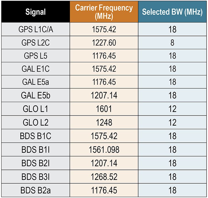
All the signals were mixed to a common intermediate frequency (IF) of 20 MHz in the recording process. Both the frequency bandwidth and the IF are fundamental to obtain the expected results from each SDR codebase. These are set in the settings file. The default configuration was validated in the testing campaign explained in later sections, and should only be modified to meet the user’s specific needs, being aware that some SDR performance characteristics may also be affected.

BASIC GNSS SDR STRUCTURE

While the general SDR receiver structure is similar across all codebases, each comes with adjustments and/or additions to adapt the code to the format of a specific signal. The general codebase structure can be summarized in four major modules:

• signal acquisition
• tracking stage
• navigation data decoding
• position, velocity and time (PVT) computation.

An important remark is that the SDR collection developed is designed to process files of limited duration. The code is designed to use enough data to provide a successful initial acquisition, and then use a single set of satellites for the remaining execution. In other words, there is no extra logic oriented at acquiring or reacquiring satellites after the first acquisition is achieved.

Signal Acquisition. The design of the acquisition scheme depends on the characteristics of the signal the SDR is aiming to process. There are numerous GNSS signal configurations for each constellation that follow different strategies concerning spreading codes, navigation data and secondary codes, which must be accounted for in the acquisition codebase.

All codebases follow a fast Fourier transform (FFT) accelerated serial search-acquisition approach to obtain estimates of the signal’s carrier frequency and code delay, where a number of signal replicas are generated iteratively, separated by a defined frequency interval in the frequency domain. All the frequency offsets are arranged in what are known as frequency bins. This frequency separation will be referred to as the frequency step. The latter is inversely proportional to the integration time and tells the maximum error allowed in the carrier frequency estimate, which is half the frequency step. Both the frequency step and the coherent integration time are parameters that have a strong effect in acquisition results, as will be seen below.

Each local replica is correlated with the input signal to obtain a code-phase estimate. The length of this correlation is the so-called coherent integration time. The maximum correlation measurement from all frequency bins is then divided by the second maximum found. This ratio is called the peak metric and is used in all SDRs to give a measure of the magnitude difference between the maximum obtained and the remaining correlation results. If the peak metric is not high enough, this implies that the maximum is close to other cross-correlation products and so could not correspond to the result obtained after correlating both input and local replica signals with the right code-phase alignment. When the peak metric surpasses the threshold defined in initSettings.m, the satellite is considered to be acquired. 

It is worth noting that in all SDR implementations the local replica is constructed by concatenating a whole primary code and a block of zeros of the same length. This prevents navigation bit transitions from affecting the correlation results. For example, GPS L2C-CM SDR’s acquisition correlates 40 milliseconds of data with 20 milliseconds of pseudorandom noise (PRN) spreading code followed by 20 milliseconds of zeros (the zero padding technique). 

Tracking Stage. The tracking stage is oriented at refining and keeping track of the code and carrier estimates provided by the acquisition stage as well as demodulating the navigation data. This is achieved using feedback loops organized in channels, which are typically referred to as tracking channels. There will be as many tracking channels as the number of satellites acquired. Each tracking channel makes adjustments to the corresponding local signal replica for the given satellite, so that it resembles the real received signal as much as possible. When the replica is sufficiently accurate, the tracking loop locks onto the signal, removes the carrier and spreading code components, and starts registering data bit transitions. The task of every tracking channel is to account for signal variations so that they can keep locked on the signal for as long as the satellite is available for use.

Tracking channels implement two feedback loops, the delay lock loop (DLL) and the Costas phase lock loop (PLL). The former is focused on the signals’ code phase while the latter on the carrier phase. These modules depend on two major parameters that determine the properties of the loop filter: the damping ratio and the noise bandwidth. On the one side, the damping ratio controls how fast the filter reaches the settling stage. On the other side, the noise bandwidth informs the amount of noise allowed in the filter.

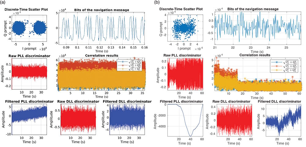
While all SDRs follow similar tracking loop schemes, some signals, such as GPS L2C, need some adjustments to the parameters mentioned above so that they provide the expected results, as we point out later. Tracking results are stored in a Matlab .mat file, but also can be assessed in the plot the tracking stage generates after it finishes processing all the channels.

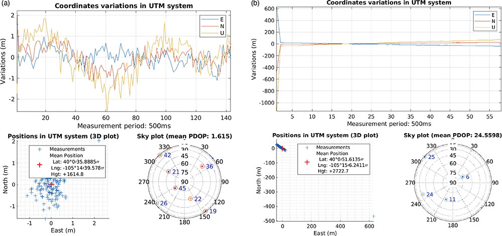
FIGURES 1a and 1b show an example of two different tracking results plots, each of which include seven figures. These show the in-phase/quadrature (I/Q prompts), the navigation data bits decoded, the changes in the raw/filtered Costas loop and DLL discriminators, and the early-prompt-late metrics. Note that the plots in Figure 1a suggest the navigation data bits were demodulated successfully. In contrast, in Figure 1b, data bits cannot be distinguished because the tracking stage failed to demodulate the navigation message.

Figure 1. (a) shows the plot generated for a successful tracking channel. In contrast, (b) illustrates the results obtained when the tracking loop in question did not lock appropriately to the signal and therefore was not able to demodulate navigation data. (Image: Authors)

Navigation Data Decoding. This stage extracts the navigation data required by the SDR codebase to compute PVT estimates from the results delivered by the tracking stage. The latter outputs I/Q prompt samples representing data bits, containing the encoded navigation data. The navigation data format for each signal can be found in the interface control document issued by each satellite constellation operator.

The general process that each SDR implements to demodulate navigation data from I/Q samples is summarized as follows:

1. detect a preamble within data bits
2. arrange the bit sequence in the corresponding structures, such as frames
3. remove secondary code if present
4. de-interleave and decode
5. check if the bit stream has errors
6. extract navigation parameters

Once navigation parameters are extracted, they are stored and later used by the functions involved in the PVT computation stage.

PVT Computation. The PVT stage takes the decoded navigation data, computes satellite positions, and solves the geometry problem, whose solution is the receiver’s location.

As with all the other stages, all SDRs follow the same approach, and use the least-squares method to solve for a position estimate once all the data is available. Position estimates are delivered in both Earth-centered Earth-fixed and east-north-up coordinates.

Similarly to the tracking stage, the PVT computation stage returns a plot showing some PVT statistics to help the user get an idea of the PVT performance of the test conducted. FIGURES 2a and 2b show an example of two positioning plots obtained for two different data files. 

Figure 2. (a) shows the plot of a priori, good statistics for the navigation solution; (b) shows a navigation plot for a file that presented a problem affecting the PVT solution. (Image: Authors)

EXPERIMENTAL SET-UP AND TESTING

In this section, we present the equipment we used in our tests (see FIGURE 3) and detail the process we followed to collect GNSS data, as well as the testing framework designed to exercise the SDR collection. 

Figure 3: The antenna was connected to the RF port of the USRP. The USRP sampled the analog data delivered by the antenna using the TCXO as the reference oscillator. The resulting sampled data was stored in a Linux-based computer.
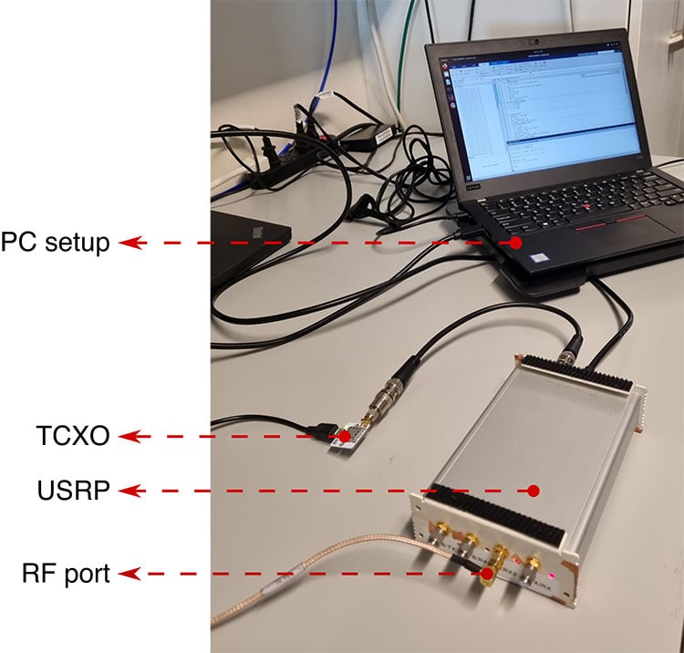
(Image: Authors)

RF Antenna. The device used to sense the RF GNSS signals was a Trimble Zephyr2 antenna, which has enhanced capabilities for multipath minimization as well as low-elevation-angle satellite tracking properties. 

The antenna was installed on the rooftop of the Ann and H.J. Smead Department of Aerospace Engineering Sciences building at the University of Colorado Boulder.

USRP and TCXO Devices. An Ettus Universal Software Radio Peripheral (USRP) B200 hardware SDR connected to an IQD temperature-compensated crystal oscillator (TCXO) was used to collect digital samples from GNSS analogue signals sensed by the antenna.

The B200 device was controlled by means of the USRP hardware driver (UHD) through a computer running a Linux operating system. UHD is a software application programming interface (API) that enables the development of code to manage USRP settings and operation. 

PC Setup. The PC setup consisted of a Linux computer  with all the required drivers and program dependencies, as well as with Mathworks’ Matlab software installed. Matlab was used to program and automate the data recording process.

Recording Process. The equipment described in previous subsections was used to record data suitable for each SDR codebase. The process to obtain signal data for all 12 codebases was reduced to eight stages by selecting an adequate frequency bandwidth, as some signals share the same central carrier frequency (see Table 2).

For each stage, a total of 100 files with 61 seconds of I/Q GNSS data were recorded over a 24-hour time period. The I/Q samples recorded by the USRP were formatted as 8 bit sine carriers. All the data sets recorded are available together with a description file based on the Institute of Navigation’s metadata standard for GNSS.

TESTING FRAMEWORK

The workflow we followed to test every codebase from the collection is outlined in the following steps:

1. Record data samples. A set of one hundred files were recorded with 61 seconds of GNSS data.
2. Debug the SDR with the selected files. A debugging stage preceded every test case to ensure the codebase performed well enough, or else to make the required adjustments.
3. Run the SDR for one hundred trials. A total of one hundred tests, one per file, were performed for all SDRs.
4. Log metrics and present results. The results from all SDR stages (acquisition, tracking and data demodulation) were stored for each file. Also, each iteration returned a message that summarized the execution results.

All of the messages returned for every file corresponded to one of the cases summarized as follows:

1. Codebase issue. Message type returned when the codebase failed because of a coding issue.
2. No navigation solution. The codebase was not able to deliver a navigation solution either due to a malfunction of the codebase or due to a lack of satellite availability. Navigation solutions are only available when both the tracking channel and the navigation data demodulation stages are successful for more than three satellites.
3. Navigation solution with accuracy worse than 30 meters. A position solution fix more than 30 meters (in three dimensions) from the known antenna location was considered a non-accurate estimate.
4. Navigation solution with accuracy under 30 meters. When the 3D positioning error was < 30 meters, the navigation solution for the position was considered accurate.

All codebases passed a debugging stage before being tried with the whole set of available data. This was done to ensure that they performed as expected, and were able to achieve the required performance in terms of the metrics mentioned above in this section. An example of this debugging stage will be explained in further detail below. We take the GPS L2C codebase as an example of how all implementations were assessed in an attempt to improve their initial performance and make them more robust to code errors. See our proceedings paper for further details of our test cases.

GPS L2C Test Case. The problem observed for GPS L2C was that some satellites acquired with a high acquisition metric were failing the tracking stage. The result was that no navigation data was demodulated from them. An in-depth study was required to find out the adjustments needed in the codebase that would help to solve this issue.

The GPS L2C signal encompasses two signal components called civil moderate (CM) and civil long (CL). The CM component is formed by a spreading code that modulates a navigation message. The CL component is a pilot (data-less) signal modulated with a longer spreading code allowing for longer coherent and non-coherent integration times, yielding better sensitivity. 

For CM signal acquisition, the 20 millisecond code length limits the coherent integration time to 20 milliseconds, due to the overlaid navigation message. This integration time defines the minimum frequency resolution required to obtain the expected correlation results. The CL component is used in the SDR to accumulate consecutive correlation results non-coherently, contributing to the receiver’s sensitivity by allowing it to operate with higher acquisition metrics in general.

The initial configuration for this SDR codebase is represented in TABLE 3a.

Table 3. Configurations for GPS L2C test case.

With this configuration, a total of 10 satellites were acquired. However, it was observed that for some satellites acquired with high peak metrics, it was not possible to demodulate their navigation data, and thus they were not considered for the navigation solution in later stages. This situation was abnormal, as typically this behavior is more characteristic of weaker signals whose bit transitions are too noisy to be decoded. This problem suggested that either the code-phase or the carrier frequency estimates (or both) were not accurate enough for each tracking channel to generate a proper replica to lock onto the input signal.

The first step taken to address this matter was to inspect the SDR’s acquisition stage for a file presenting the mentioned problems. For instance, taking a closer look at the carrier and code-phase 3D representation for those satellites acquired with a high acquisition metric that were not successfully tracked afterwards. After doing so, some satellites were identified with the irregular characteristics described above, as for example the PRN 10 satellite. PRN 10 is taken as a reference throughout this subsection.

The metric analyzed for PRN 10 was the matrix built by the acquisition’s serial search process. This matrix contains the correlation results obtained for each frequency bin. The width of each frequency bin is determined by the frequency step size defined in the configuration file. In this way, the smaller the frequency step, the more frequency bins that the corresponding matrix contains. This implies a better frequency resolution. 

With this in mind, the frequency resolution was progressively increased by decreasing the frequency step size. Extra logic had to be added to the acquisition algorithm to implement this feature. It was found that when using a step size of 6.5 Hz, the tracking stage was then able to lock and demodulate navigation bits from PRN 10 effectively. This was the most significant determining factor to overcome the issue in question for the majority of the satellites available. However, other smaller adjustments also improved tracking results in general. These are depicted in TABLE 3b.

CODE AVAILABILITY

All the resources concerning the SDR collection are publicly available at the portal hosted by University of Colorado Boulder. Through this portal, all the GNSS codebases along with the data sets for testing can be acquired, as well as access to the discussion forum.

CONCLUSION

The first version of the SDR collection was made available after the seminal text by Borre et al. was published and consisted of a GPS L1C/A SDR and multiple data sets. From then on, this project kept evolving by adding more SDRs as new GNSS signals emerged across different satellite constellations.

Our most recent work was to collect all the SDR codebases, arrange them in a common format, and test each implementation to assert their robustness and extract statistics concerning their performance.

Future work will be dedicated to adding more features aiming at refining the PVT estimates delivered by each SDR.

More progress is expected to be made soon, with additional improvements made in the GNSS laboratory. In addition, there is plenty of room for contributions from other researchers who want to support and collaborate with this open-source initiative. Our portal provides a convenient way to manage these contributions.

ACKNOWLEDGMENTS

We thank the many individuals who collaborated in the development of the open-source GNSS SDR collection. 

This article is based on the paper “A Collection of SDRs for Global Navigation Satellite Systems (GNSS)” presented at ION ITM 2022, the 2022 International Technical Meeting of the Institute of Navigation, Jan. 25–27, 2022. 

JOAN BERNABEU is a Ph.D. student at the Institut Supérieur de l’Aéronautique et de l’Espace, Toulouse, France. He also works as a satellite navigation engineer for GMV, Spain.

NICOLAS GAULT is a Ph.D student at École Nationale d’Aviation Civile, Toulouse, France. He was a visiting scholar in the Department of Aerospace Engineering Sciences at the University of Colorado (CU) Boulder in 2020-2021.

YAFENG LI is an associate professor in the School of Automation at the Beijing Information Science and Technology University, China. He was a visiting researcher with the Department of Aerospace Engineering Sciences, CU Boulder in 2017–18.

DENNIS M. AKOS is a faculty member in the Department of Aerospace Engineering Sciences at CU Boulder.