No audio available for this content.
A GPS-lidar fusion technique implements a novel method for efficiently modeling lidar-based position error covariance based on features in the point cloud. The fusion uses a three-dimensional (3D) city model to detect and eliminate non-line-of-sight (NLOS) GPS satellites to improve global positioning.
The technique has potential application in UAV missions such as 3D modeling, filming, surveying, search and rescue, and package delivery.
By Akshay Shetty and Grace Xingxin Gao, University of Illinois
Unmanned aerial vehicles (UAVs) commonly rely on GPS for continuous and accurate outdoor position estimates. However, in certain urban scenarios, additional onboard sensors such as light detection and ranging (lidar) are desirable due to errors in GPS measurements. To fuse these measurements it is important, yet challenging, to accurately characterize their error covariance. We propose a GPS-lidar fusion technique with a novel method for efficiently modeling the position error covariance based on surface and edge features in point clouds. We use the lidar point clouds in two ways: to estimate incremental motion by matching consecutive point clouds; and, to estimate global pose (position and orientation) by matching with a 3D city model. For GPS measurements, we use the 3D city model to eliminate NLOS satellites and model the measurement covariance based on the received signal-to-noise-ratio (SNR) values. Finally, all the above measurements and error covariance matrices are input to an unscented Kalman Filter (UKF), which estimates the globally referenced pose of the UAV. To validate our algorithm, we conducted UAV experiments in GPS-challenged urban environments on the University of Illinois at Urbana-Champaign campus.These experiments demonstrate a clear improvement in the UAV’s global pose estimates using the proposed sensor fusion technique.
SITUATION
Emerging applications in UAVs such as 3D modeling, filming, surveying, search and rescue, and package delivery all involve flying in urban environments. In these scenarios, autonomously navigating a UAV has certain advantages such as optimizing flight paths and sensing and avoiding collisions. However, to enable such autonomous control, we need a continuous and reliable source for UAV positioning. In most cases, GPS is primarily relied on for outdoor positioning. However, in an urban environment, GPS signals from the satellites are often blocked or reflected by surrounding structures, causing large errors in the position output.
In cases when GPS is unreliable, additional onboard sensors such as lidar can provide the navigation solution. An onboard lidar provides a real-time point cloud of the surroundings of the UAV. In a dense urban environment, lidar can detect a large number of features from surrounding structures such as buildings.
Positioning based on lidar point clouds has been demonstrated primarily by applying different simultaneous localization and mapping (SLAM) algorithms. In many cases, algorithms implement variants of iterative closest point (ICP) to register new point clouds.
APPROACH
The main contribution of this article is a GPS-lidar fusion technique with a novel method for efficiently modeling the error covariance in position measurements derived from lidar point clouds. Figure 1 shows the different components involved in the sensor fusion.

We use the lidar point clouds in two ways: to estimate incremental motion by matching consecutive point clouds; and, to estimate global pose by matching with a 3D city model. We use ICP for matching the point clouds in both cases.
For the lidar-based position estimates, we proceed to build the error covariance model depending on the surrounding point cloud. First, we extract surface and edge feature points from the point cloud. We then model the position error covariance based on these individual feature points. Finally, we combine all the individual covariance matrices to model the overall position error covariance ellipsoid.
For the GPS measurement model, we use the pseudorange measurements from a stationary reference receiver and an onboard GPS receiver to obtain a vector of double-difference measurements. Using the double-difference measurements eliminates clock bias and atmospheric error terms, hence reducing the number of unknown variables. We use the global position estimate from the lidar-3D city matching to construct LOS vectors to all the detected satellites. We then use the 3D city model to detect NLOS satellites, and consequently refine the double-difference measurement vector. We create a covariance matrix for the GPS double-difference measurement vector based on SNR of the individual pseudorange measurements.
We implement a UKF to integrate all lidar and GPS measurements. Additionally, we incorporate orientation, orientation rate and acceleration measurements from an onboard inertial measurement unit (IMU). Finally, we test the filter on an urban dataset to show an improvement in the navigation solution.
LIDAR-BASED ODOMETRY
ICP is commonly used for registering three-dimensional point clouds. It takes a reference point cloud q, an input point cloud p, and estimates the rotation matrix R and the translation vector T between the two point clouds. Different variants of the algorithm generally consist of three primary steps.
Matching. This involves matching each point pi in the input point cloud, to a point qi in the reference point cloud. The most common method is to find the nearest neighbors of each point in the input point cloud. For our application, a kDtree performs best since the two point clouds are relatively close to each other.
Defining Error Metric. This defines the error metric for the point pairs. We choose the point-to-point metric, which is generally more robust to difficult geometry than other metrics such as point-to-plane. The total error between the two point clouds is defined as follows:
![]() (1)
(1)
where N is the number of points in the input point cloud p.
Minimization. The last step of the algorithm is the minimization of the error metric with regard to the rotation matrix R and the translation vector T between the two point clouds.
We use ICP to estimate the incremental motion of the lidar between consecutive point clouds. Figure 2 shows our implementation of ICP to estimate the lidar odometry.

MATCHING LIDAR, 3D MODEL
We generate our 3D city model using data from two sources: Illinois Geospatial Data Clearinghouse and OSM. The Illinois Geospatial Data were collected by a fixed-wing aircraft flying at an altitude of 1700 meters, equipped with a lidar system including a differential GPS unit and an inertial measurement system to provide superior global accuracy. Since the data were collected from a relatively high altitude, it primarily contains adequate details for the ground surface and the building rooftops. In order to complete the 3D city model, we need additional information for the sides of buildings. We use OSM to obtain this information. OSM is a freely available, crowd-sourced map of the world, which allows users to obtain information such as building footprints and heights. Figure 3 shows a section of the 3D city model for Champaign County.

To estimate the global pose of the lidar, we match the onboard lidar point cloud with the 3D city model using ICP, in these steps:
- Use the position output from onboard GPS receiver as an initial guess. If position output is unavailable, use the position estimate from the previous iteration as an initial guess. For orientation, use the estimate from the previous iteration. Thus, we obtain an initial pose guess
 .
. - Project the onboard lidar point cloud pL to the same space as the 3D city model qcity using .
- Implement ICP, to obtain the rotation RL and translation TL between the two point clouds. Use this output to obtain an estimate for the global pose
 .
.
Figure 4 shows the results of implementation of the above method. While navigating in urban areas, the GPS receiver position output used for the initial pose guess![]() might contain large errors in certain directions. This might cause ICP to converge to a local minimum, depending on features in the point cloud pL generated by the onboard lidar.
might contain large errors in certain directions. This might cause ICP to converge to a local minimum, depending on features in the point cloud pL generated by the onboard lidar.

To evaluate how our lidar-3D city model matching algorithm performs in such challenging cases, we test it in two different urban areas as shown in Figure 5. We begin by selecting a grid of initial position guesses up to 20 meters away from the true position. With an adequate distribution of features, ICP is able to correctly match the two point clouds and provide an accurate position estimate after matching. In contrast, when there’s an urban scenario with a relatively poor distribution of features, ICP is unable to estimate the position accurately.

MODELING ERROR COVARIANCE
We model the lidar position error covariance as a function of the surrounding features. In urban environments, we typically observe structured objects such as buildings, hence we focus primarily on surface and edge features in the point cloud. We extract these feature points based on the curvature at each point. Points with curvature values above a threshold are marked as edge points, whereas points with curvature values below a threshold are marked as surface points. (For detailed discussion of the algorithms involved, see GPS-LiDAR_AkshayShetty-algorithms.
For each surface feature point, we first compute the normal by using 9 of the neighboring points to fit a plane. We model the error covariance ellipsoid with the hypothesis that each surface feature point contributes in reducing position error in the direction of the corresponding surface normal. Additionally, we assume that surface points closer to the lidar are more reliable than those further away, because of the density of points.
For each edge feature point, we first find the direction of the edge using the closest edge points in the scans above and below. We model the error covariance ellipsoid with the hypothesis that each edge feature point helps in reducing position error in the directions perpendicular to the edge vector. A vertical edge, for example, would help in reducing horizontal position error. Additionally, we assume that edge points closer to the lidar are more reliable than those further away, again because of the density of points. Figure 6 shows sample error covariance ellipsoids for a surface point and an edge point.

To obtain the overall position error covariance, we combine the error covariance matrices for all the individual surface and edge feature points. Figure 7 shows the combined covariance ellipsoid for two different scenarios. We observe that while passing through a corridor, the covariance ellipsoid is larger in the direction parallel to the building sides due to a poor distribution of features.

GPS MEASUREMENT MODEL
We use pseudorange measurements from the GPS receiver to create the measurement model. To eliminate certain error terms, we use double-difference pseudorange measurements, which are calculated by differencing the pseudorange measurements between two satellites and between two receivers. Before proceeding to use the pseudorange measurements, we check if any of the satellites detected by the receiver are NLOS signals. We use the 3D city model mentioned earlier to detect the NLOS satellites. We use the position output generated by the lidar-3D city model matching to locate the receiver on the 3D city model.
Next, we draw LOS vectors from the receiver to every satellite detected by the receiver and eliminate satellites whose corresponding LOS vectors intersect the 3D city model. Figure 8 shows the above implementation in an urban scenario.

After eliminating the NLOS satellites, we select satellites that are visible to both the user and the reference receivers to create the GPS double-difference measurement vector and its covariance. We assume that the individual pseudorange measurements are independent, and that the variance for each measurement is a function of the corresponding SNR. We propagate the covariance matrix for the individual pseudorange measurements, to obtain the covariance matrix for the double-difference measurements.
GPS-Lidar Integration
In addition to using a lidar and a GPS receiver, we use an IMU on board the UAV. Figure 9 shows the experimental setup: the UAV designed and built by our research group. For the double-difference GPS measurements, we use a reference receiver within a kilometer of our data collection sites. We implement a UKF to fuse measurements from the sensors and estimate the global pose of the UAV.

Position and orientation estimates from lidar and GPS are incorporated via the correction step of the filter, whereas the IMU measurements are included in the prediction step. For position corrections from lidar, we use our point cloud feature based model for the error covariance. For GPS double-difference measurements, we use the covariance based on the individual pseudorange measurement SNR.
We implement our algorithm on an urban dataset collected on our campus of University of Illinois at Urbana-Champaign. As shown in Figure 10, the GPS measurements and the GPS position output contain large errors, due to the presence of nearby urban structures. Here we stack all the double-difference measurements and compute the unweighted least square estimate of the baseline between the UAV and the reference receiver.

For the lidar measurements, we check the output from our incremental ICP odometry method and the lidar-3D city model matching algorithm. Furthermore, we implement an ICP mapping algorithm to check the performance of existing ICP-based methods on the dataset. In Figure 11, the ICP odometry method and the ICP mapping algorithm accumulate drift over the course of the trajectory. The lidar-3D city model matching algorithm does not drift over time; however, the position still contains errors in situations where the lidar does not detect enough number of points or the matching algorithm converges to a local minimum.

Figure 12 shows the output of the filter for the same trajectory. The filter output estimates the actual path much more accurately than the individual measurement sources by themselves.

CONCLUSION
In summary, we proposed a GPS-lidar integration approach for estimating the navigation solution of UAVs in urban environments. We used the onboard lidar point clouds in two ways: to estimate the odometry by matching consecutive point clouds, and to estimate the global pose by matching with an external 3D city model. We built a model for the error covariance of the lidar-based position estimates as a function of surface and edge feature points in the point cloud. For GPS measurements, we eliminated NLOS satellites using the 3D city model and used the remaining double-difference measurements between an onboard receiver and a reference receiver. To construct the covariance matrix for the double-difference measurements, we used the SNR values for individual pseudorange measurements.
Finally, we applied an UKF to integrate the measurements from lidar, GPS and an IMU. We experimentally demonstrated the improved positioning accuracy of our filter.
ACKNOWLEDGMENTS
The authors would like to sincerely thank Kalmanje Krishnakumar and his group at NASA Ames Research Center for supporting this work under the grant NNX17AC13G.
The material in this article was first presented at the ION GNSS+ 2017 conference in Portland, September 2017.
MANUFACTURERS
The lidar used aboard the UAV in these tests is a Velodyne VLP-16 Puck Lite. The GPS receiver is a u-blox LEA-6T with a Maxtena M1227HCT-A2-SMA antenna. The IMU is an Xsens Mti-30, and the onboard computer an AscTec Mastermind 3a.
The iBQR UAV was designed and assembled by the authors.
AKSHAY SHETTY received an M.S. degree in aerospace engineering from University of Illinois at Urbana-Champaign. He is also pursuing a Ph.D. at the same university.
GRACE XINGXIN GAO received a Ph.D. degree in electrical engineering from Stanford University. She is an assistant professor in the Aerospace Engineering Department at the University of Illinois at Urbana-Champaign.