No audio available for this content.
When a platform’s mission requires maneuvering among different environments, transitions between these environments may mean that a single method cannot solve the full positioning, navigation and mapping problem.
This article describes an integrated navigation and mapping design using a GPS receiver, an inertial measurement unit, a monocular digital camera and three short-to-medium range laser scanners.
By Evan T. Dill and Steven D. Young, NASA Langley Research Center, and Maarten Uijt de Haag, Ohio University
An unmanned aircraft system (UAS) traffic management system (UTM) is an ecosystem for coordinating UAS operations in uncontrolled airspace, particularly operations under 400 feet altitude involving small- to mid-sized vehicles. In this domain, information services regarding the state of the airspace will be provided to UAS operators.
In addition, UTM would coordinate and authorize access to airspace for particular time periods based on requests from the operators. The Federal Aviation Administration would maintain regulatory and operational authority, and may for example, issue changes to constraints or airspace configurations to operators via this information service. However, there is no direct control from air traffic control personnel (such as “climb and maintain 300 feet” or “turn left, heading 150”).
As with visual flight rules operations of manned aircraft in uncontrolled airspace, under UTM the onus is on the vehicle operator to assure the flight system provides adequate performance with regard to communication, navigation and surveillance during flight. The vehicle/operator is responsible for avoiding other aircraft, terrain, obstacles and incompatible weather. UTM information services do not yet include, for example, information from an alternative positioning, navigation and timing system that may be needed for operations conducted in GPS-degraded environments (such as near buildings or other structures). This is the challenge being addressed by the integrated navigation concept described in this article. Other concepts are also being considered and developed for alternate, and unique, UAS missions and flight environments.
The method presented here employs a monocular camera as part of a multi-sensor solution that continuously operates throughout and between outdoor and structured indoor environments. For this work, an indoor environment is considered “structured” if its walls are vertical and remain approximately parallel, while the floor is either roughly flat or slanted.
In this type of environment, GPS is typically only sparsely available or not available at all. Hence, in our proposed navigation architecture, additional information from a camera and multiple laser range scanners (not the focus of this article) are used to increase the system’s positioning, navigation and mapping availability and accuracy in a GPS-challenged indoor environment. Figure 1 shows the target operational scenario, and Figure 2 the equipped multi-copter used in this research.


Figure 3 shows a block diagram for the methodology implemented in this research, with the elements related to monocular camera methods highlighted. When assessing the capabilities of each of the sensors used in the work, only the inertial sensor produces data that is solely dependent on the motion of the platform and local gravity and is more or less unaffected by its surroundings. Therefore, the inertial is chosen to be the primary sensor for this method.
The mechanization integrates the measurements from GPS, the laser scanners and the monocular camera through a complementary Kalman Filter (CKF) that estimates the errors in the inertial measurements and feeds them back to the inertial strapdown calculations. For this inertial error estimation method to function properly, pre-processing methods must be implemented that relate the sensors’ observables to the inertial measurements.
Here we describe the processing techniques necessary to relate measurements from a monocular camera to measurements from the inertial measurement unit (IMU). Then we show how these techniques are used in the broader GPS/optical/inertial mechanization and present testing results.

2D Monocular Camera Methods
To process data from the camera, we first perform feature detection and tracking of both point features and line features. Specifically, elements from Lowe’s Scale Invariant Feature Transforms (SIFT) are used to track point features, which are in turn used to obtain estimates of the camera’s rotational and un-scaled translational motion using structure from motion (SFM) based methods. To resolve the ambiguous scale factor, a novel scale estimation technique is employed that uses data from the platform’s horizontally scanning laser. This technique as well as algorithms that produce a 3D visual odometry solution are presented below.
SIFT Point Feature Extraction. To aid in determining camera motion, SIFT has been used as a way of identifying local features that are invariant to translation, rotation, and image scaling. This technique yields 2D point features that are unique to their surroundings and readily identified and associated across a set of sequential camera images. Each key location and its surroundings are analyzed, resulting in a descriptive 128-element feature vector, known as a SIFT key. Example results of the SIFT key identification process are shown in Figure 4.

Based on the results of the SIFT feature extraction process from two image frames, a feature association function is performed using the feature vectors. For this work, a two-step procedure is implemented.
First, SIFT keys are associated using a matching procedure. Example results of this process are shown in Figure 5, where it can be observed that incorrectly associated features may result from this process. To remove these artifacts, inertial measurements are utilized to ensure the correctness of the associations.

Using a triangulation method, prospective associations are used to crudely estimate each feature’s 3D position with respect to the previous frame. While this triangulation method yields 3D data, it is of poor quality, and is therefore only used to obtain rough approximations that are sufficient for association purposes, but insufficient for navigation purposes.
Once transformed to a 3D reference frame, the projected distances of each feature are compared with one another, and prospective associations that produce significantly different depths than surrounding points are eliminated. Example results of this filtering process can be seen in Figure 6.

In future implementations, the ORB feature will be evaluated, as its performance is expected to be more than two orders of magnitude faster than SIFT.
Wavelet Line Feature Extraction. To implement the scale factor estimation technique described in a later section, it is necessary to first extract and track vertical line features. To accomplish this, a method using wavelet transforms (WTs) was developed. When applied to a 2D image, WTs can be viewed as filters operating in the x and y directions of an image. By applying either a high- or low-pass filter to both of an image’s channels (that is, x and y directions), four sub-images are formed to represent an image approximation. For this work, a level-one bi-orthogonal 1.3 wavelet was used to decompose each image. An example of the four sub-images produced by this wavelet is shown in Figure 7 along with the original image.

Through further processing of the vertical decomposition results, strong line features are identified by first inspecting the illuminated elements along the vertical channels of the decomposed image and identifying clusters of adjacent pixels. Next, a 2D line fit is applied to the groups to estimate residual noise. Pixel collections with low residuals (<3 here) are considered valid line features. Example results of this process are shown in Figure 8.

For association purposes, lines cannot be compared over a sequence of image frames solely based on location as similar line features may not necessarily possess the same endpoint, and, therefore, can be of varying lengths. However, corresponding lines will possess many common points and similar orientations if they are projected into the same frame. Using the inertial reference frame, each line’s orientation, ![]() , can be transformed across image frames as given by:
, can be transformed across image frames as given by:
![]()
In this manner, lines between frames that contain multiple similar points and have comparable orientations are considered associated.
For a discussion of the projective visual odometry and epipolar geometry methodology as well as the resolution of true metric scale used in this work, download the supplemental PDF.
Metric Scale. As the unscaled translation estimate calculated through the aforementioned visual odometry method is a unit vector, it only indicates the most likely direction of motion of the camera. To obtain the sensor’s actual translational motion, an estimate of the scale factor, m, is required to determine the absolute translation ∆r. This can be accomplished through techniques using a priori knowledge of the operational environment or measurements from other sensors. In this research effort, a new method is employed that makes use of data provided by a horizontally scanning laser.
The proposed method estimates the scale in an image by identifying points in the environment that are simultaneously observed by the camera and the forward-looking laser range scanner.
To enable this estimation method we must identify the correspondences between the pixels in the camera images (each defined by a direction unit vector corresponding to the row x and column y) and the laser scanner measurements (each defined by direction unit vector). A calibration procedure establishes these correspondences. Given the laser range measurements, 2D features located on the scan/pixel intersections can be scaled up to 3D points.
Unfortunately, extracted 2D point features are rarely illuminated by a laser scan in two consecutive frames. This can be resolved by considering the intersection of a laser scan with 2D line features rather than point features. As the laser intersects the camera frame at the same location regardless of platform motion, and the platform does not make excessive roll and pitch maneuvers, vertical line features in the image frame are preferred as they will be relatively orthogonal to the laser scan plane.
Using the previously described vertical line extraction procedure, Figure 9 shows an example image frame overlaid with the points in the image frame illuminated by the laser (indicated by a blue line) and the extracted vertical line features (indicated as green lines). Multiple intersections of 2D vertical lines with laser scan data are calculated (indicated as red points). Inversely, Figure 10 depicts the location of all laser scan points in green, all laser points observable with the camera field-of-view (FoV) in blue, and intersection points in red.


For scale factor calculation purposes, it is necessary to track the motion of these 3D laser/vision intersection points, across sequences of camera image frames. As each intersection point uniquely belongs to a line feature in the 2D image frame, it can be stated that if two lines are associated, their corresponding intersection points are also associated. Using the rotation computed from the visual odometry process, the line association method described by (1) is implemented, and provides associations between laser/vision intersection points across frames.
To calculate the desired scale factor based on these associated laser/vision points, geometric relationships are established: unit vectors from the camera center to points located on a 2D line. From these, the line’s normal vector can be derived.
Monocular Camera Results
To assess the performance of the visual odometry processes, multiple experiments were conducted. The results of one such test are discussed here. During each test, the visual odometry results for rotation, shown in blue, were easily evaluated through comparison with the platform’s inertially-measured rotation, displayed in red.
The rotational results for each sensor were decomposed into the Euler angles: pitch, roll and yaw with respect to an established navigation frame. Unfortunately, the inertial sensor itself cannot be used to evaluate the visual odometry translation results due to relatively large inertial drift in the sensor measurements. As no independent measurements were available to evaluate translation with high precision, the truth reference was established by accurately measuring the actual paths taken during each flight.
A test flight was conducted traversing a rectangular indoor hallway loop. This test contained translation in multiple dimensions, large heading changes and a flight duration of four minutes. Moreover, this test allowed for evaluation of the eight-point algorithm and scale estimation method in the presence of rapid scene changes.
The attitude estimation results for this test are shown in Figure 11. Throughout data collection, the maximum separation between the inertial and vision-based attitude estimators for pitch, roll and yaw was 9°,19° and 14°, respectively. Upon comparison to many of the other conducted tests, the maximum attitude errors were larger. There are multiple reasons for this increase. First, the duration of this experiment was greater than that of previous experiments. Errors accumulate as a function as time due to integration of residual bias errors, so increasing flight duration will increase cumulative error.

Next, the looping path observed throughout this test caused the eight-point algorithm and scale estimation procedures to quickly adapt to differing scenery. Drastic scene changes (turning a corner) increase the difficulty of feature association between frames. This directly affects the procedures used for visual odometry in an adverse manner. Finally, there are situations in this flight where features are sparse. In general, a decrease in features will cause a decrease in the estimation capabilities of visual odometry.
Figure 12 shows the visual odometry path calculated for experiment 2. Here, the estimated length of each of the four straight legs of the rectangular loop matches to within 2 meters of the measured hallway lengths. This implies that the scale estimation technique is working reasonably well.

As for the estimated translational directionality produced by the eight-point algorithm, the first two legs of the loop never divert from the measured path by more than 2 meters; the third leg diverts by 5 meters. This is most likely due to a lack of well dispersed features in that specific hallway.
The cumulative error contained in the third linear leg of the loop also makes evaluation of the final leg difficult. However, if previous errors are removed, the final leg appears to match the measured path well. In total, the landing position calculated through visual odometry is 6.5 meters away from the measured end of the trial.
Integration Methodology
In cases where GPS measurements are available along with the visual odometry solution, the proposed method can extend the GPS/IMU integration mechanization. The structure of the referenced GPS/inertial integration consists of two filters: a dynamics filter that uses GPS carrier-phase measurements to estimate velocity and other IMU errors, and a position filter that uses the velocity output of the dynamics filter and GPS pseudoranges. The dynamics filter can be adapted and extended to include camera data within its mechanization.
The dynamics filter is a CKF designed to estimate the inertial error states: velocity error in the north-east-down (NED) coordinate reference frame, misorientation (including tilt error), gyro bias error, and specific force or accelerometer bias error. This yields a state vector. For a discussion of the state vector, download the supplemental PDF.
Results
To evaluate the proposed algorithms, data was collected through multiple flights of the hexacopter platform shown in Figure 2 through a structured indoor and outdoor environment including transitions between these two environments. The availability of GPS measurements in these environments ranged from fully denied, to substantially degraded, to enough observables for a full solution.
The results of one test flight are discussed in this section. Apart from the data collections with the hexacopter, truth reference maps were created for the indoor operational environment and used for evaluation of the described processes. The results of the full GPS/inertial/laser/camera integrated solution described in Figure 3 are shown in an NED frame in Figure 13.

The truth reference of the environment, depicted in red (derived from a terrestrial laser scanner), is compared to the flight path obtained from the extended Kalman filter (EKF), displayed in blue. The estimated flight trajectory constantly remains within the hallway truth model, indicating sub-meter level performance. Furthermore, based on an extension of this work for environmental laser mapping produced from the EKF, combined with the accuracy of the map, it is further reinforced that sub-meter-level navigation performance is obtained.
During portions of the described data collection, there was enough visibility (>3 satellites) to calculate a GPS position. The availability of GPS measurements to the position estimation portion of the filter allowed for geo-referencing of the produced flight path and 3D map.
Figure 14 displays the geo-referenced continued flight path based on the integration filter superimposed on Google Earth on the left, while the standalone GPS solution based on pseudoranges only is plotted on the right. The geo-referenced path correctly displays the platform passing through Stocker Center, the Ohio University engineering building.

To demonstrate the contributions of the monocular camera to the above results, laser measurements were removed from the solution for a 20-second period where GPS was unavailable. During the 20-second removal of laser data, the system is forced to operate on integration between visual odometry measurements and the IMU. The cumulative effect caused by this situation can be observed in Figure 15. After coasting on an IMU/camera solution for 20 seconds, the path is subsequently altered by 3 meters, as opposed to the solution with all sensors.

To further emphasize the contribution of the visual odometry component, both the laser and camera were removed from the integration for the same 20-second period. During this time frame the EKF is forced to coast on calibrated inertial measurements. The effect of losing all secondary sensors for a 20-second period can be observed in Figure 16.

During the forced sensor outage, a 45-meter cumulative difference is introduced between the path using all sensors and the path with denied sensors. Through comparison of the results shown in Figure 15 and Figure 16, the contribution of monocular camera data can be isolated.
When the EKF was forced to operate for 20 seconds using an IMU/camera solution, 3 meters of error were introduced. This is significantly smaller than the 45 meters of error observed when using only the inertial for the same period. Thus, the camera is shown to provide stability to the EKF when neither the laser nor GPS are available.
Conclusions
The visual odometry techniques produced reasonably good attitude estimation and are effective at constraining inertial drift when other sensors are not available. The inclusion of camera measurements to the discussed integrated solution resulted in increases in the accuracy, availability, continuity and reliability of the system.
Acknowledgment
The material in this article was first presented at the ION Pacific PNT conference in Hawaii, May 2017.
Manufacturers
The camera used aboard the UAV in these tests is a Point Grey Firefly MV and the IMU is an XSENS MTi. The GPS receiver is a NovAtel OEMStar with a corresponding NovAtel L1 patch antenna.
EVAN T. DILL is a research scientist in the Safety Critical Avionics Systems Branch at NASA Langley Research Center. He received his Ph.D. in electrical engineering from Ohio University.
STEVEN D. YOUNG is a senior research scientist at NASA with more than 30 years of experience in the related fields of safety assurance, avionics systems engineering and human-machine interaction.
MAARTEN UJIT DE HAAG is the Edmund K. Cheng Professor of Electrical Engineering and Computer Science and a Principal Investigator (PI) with the Avionics Engineering Center at Ohio University, where he earlier earned his Ph.D. in electrical engineering.