Update: GNSS Accuracy: Lies, Damn Lies, and Statistics

By Frank van Diggelen, Global Locate, Inc.

This update to a frequently requested article first published here in 1998 explains how statistical methods can create many different position accuracy measures. As the driving forces of positioning and navigation change from survey and precision guidance to location-based services, E911, and so on, some accuracy measures have fallen out of common usage, while others have blossomed. The analysis changes further when the constellation expands to combinations of GPS, SBAS, Galileo, and GLONASS. Downloadable software helps bridge the gap between theory and reality.

“There are three kinds of lies: lies, damn lies, and statistics.” So reportedly said Benjamin Disraeli, prime minister of Britain from 1874 to 1880. Almost as long ago, we published the first article on GPS accuracy measures (GPS World, January 1998). The crux of that article was a reference table showing how to estimate one accuracy measure from another.

The original article showed how to derive a table like TABLE 1. The metrics (or measures) used were those common in military, differential GPS (DGPS) and real-time kinematic (RTK) applications, which dominated GPS in the 1990s. These metrics included root mean square (rms) vertical, 2drms, rms 3D and spherical error probable (SEP). The article showed examples from DGPS data.

Table 1. Accuracy measures for circular, Gaussian, error distributions.

Figure 1. Using Table 1.

Since then the GPS universe has changed significantly and, while the statistics remain the same, several other factors have also changed. Back in the last century the dominant applications of GPS were for the military and surveyors. Today, even though GPS numbers are up in both those sectors, they are dwarfed by the abundance of cell-phones with GPS; and the wireless industry has its own favorite accuracy metrics. Also, Selective Availability was active back in 1998, now it is gone. And finally we have the prospect of a 60+ satellite constellation, as we fully expect in the next nine years that 30 Galileo satellites will join the GPS and satellite-based augmentation systems (SBAS) satellites already in orbit.

Therefore, we take an updated look at GNSS accuracy.

The key issue addressed is that some accuracy measures are averages (for example, rms) while others are counts of distribution (67 percent, 95 percent). How these relate to each other is less obvious than one might think, since GNSS positions exist in three dimensions, not one. Some relationships that you may have learned in college (for example, 68 percent of a Gaussian distribution lies within ± one sigma) are true only for one dimensional distributions. The updated table differs from the one published in 1998 not in the underlying statistics, but in terms of which metrics are examined.

Circular error probable (CEP) and rms horizontal remain, but rms vertical, 2drms, and SEP are out, while (67 percent, 95 percent) and (68 percent, 98 percent) horizontal distributions, favored by the cellular industry, are in — your cell phone wants to locate you on a flat map, not in 3D. Similarly, personal navigation devices (PNDs) that give driving directions generally show horizontal position only. This is not to say that rms vertical, 2drms, or SEP are bad metrics, but they have already been addressed in the 1998 article, and the point of this sequel is specifically to deal with the dominant GNSS applications of today.

Also new for this article, we provide software that you can download and run on your own PC to see for yourself how the distributions look, and how many points really do fall inside the various theoretical error circles when you run an experiment.

Table 1 is the central feature of this article. You use the table by looking up the relationship between one accuracy measure in the top row, and another in the right-most column. For example (see FIGURE 1), let’s take the simplest entry in the table: rms2 = 1.41× rms1

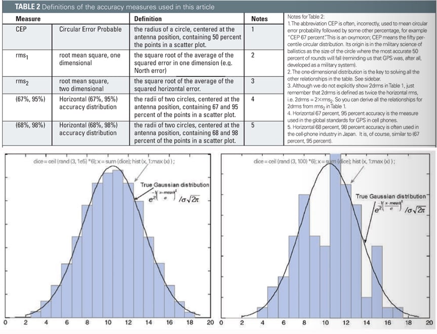
TABLE 2 defines the accuracy measures used in this article.

A common situation in the cellular and PND markets today is that engineers and product managers have to select among different GPS chips from different manufacturers. (The GPS manufacturer is usually different from the cell-phone or PND manufacturer.) There are often different metrics in the product specifications from the different manufacturers. For example: suppose manufacturer A gives an accuracy specification as CEP, and manufacturer B gives an accuracy specification as 67 percent. How do you compare them? The answer is to use Table 1 to convert to a common metric. Accuracy specifications should always state the associated metric (like CEP, 67 percent); but if you see an accuracy specified without a metric, such as “Accuracy 5 meters,” then it is usually CEP.

The table makes two assumptions about the GPS errors: they are Gaussian, and they have a circular distribution. Let’s discuss both these assumptions.

Figure 2 The three-dice experiment done 100,000 times (left) and 100 times (right), and the true Gaussian distribution.

Gaussian Distribution

In plain English: if you have a large set of numbers, and you sort them into bins, and plot the bin sizes in a histogram, then the numbers have a Gaussian distribution if the histogram matches the smooth curve shown in FIGURE 2. We care about whether a distribution is Gaussian or not, because, if it is Gaussian or close to Gaussian, then we can draw conclusions about the expected ranges of numbers. In other words, we can create Table 1. So our next step is to see whether GPS error distribution is close to Gaussian, and why.

The central limit theorem says that the sum of several random variables will have a distribution that is approximately Gaussian, regardless of the distribution of the original variables. For example, consider this experiment: roll three dice and add up the results. Repeat this experiment many times. Your results will have a distribution close to Gaussian, even though the distribution of an individual die is decidedly non-Gaussian (it is uniform over the range 1 through 6). In fact, uniform distributions sum up to Gaussian very quickly.

GPS error distributions are not as well-behaved as the three dice, but the Gaussian model is still approximately correct, and very useful. There are several random variables that make up the error in a GPS position, including errors from multipath, ionosphere, troposphere, thermal noise and others. Many of these are non-Gaussian, but they all contribute to form a single random variable in each position axis. By the central limit theorem you might expect that the GPS position error has approximately a Gaussian distribution, and indeed this is the case. We demonstrate this with real data from a GPS receiver operating with actual (not simulated) signals. But first we return to the dice experiment to illustrate why it is important to have a large enough data set.

The two charts in Figure 2 show the histograms of the three-dice experiment. On the left we repeated the experiment 100,000 times. On the right we used just the first 100 repetitions. Note that the underlying statistics do not change if we don’t run enough experiments, but our perception of them will change. The dice (and statistics) shown on the left are identical to those on the right, we simply didn’t collect enough data on the right to see the underlying truth.

FIGURE 3 shows a GPS error distribution. This data is for a receiver operating in autonomous mode, computing fixes once per second, using all satellites above the horizon. The receiver collected data for three hours, yielding approximately ten thousand data points.

Figure 3. Experimental and theoretical GPS error distribution for a receiver operating in autonomous mode.

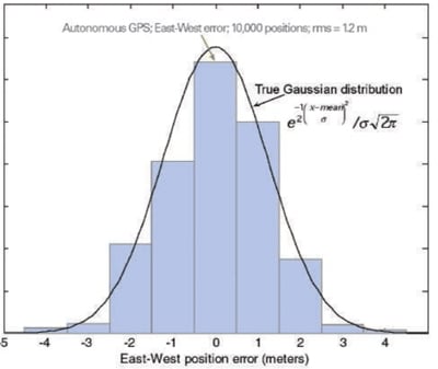
You can see that the distribution matches a true Gaussian distribution in each bin if we make the bins one meter wide (that is, the bins are 10 percent the width of the 4-sigma range of the distribution). Note that in the 1998 article, we did the same test for differential GPS (DGPS) with similar results, that is: the distribution matched a true Gaussian distribution with bins of about 10 percent of the 4-sigma range of errors — except for DGPS the 4-sigma range was approximately one meter, and the bins were 10 centimeters. Also, reflecting how much the GPS universe has changed in a decade, the receiver used in 1998 was a DGPS module that sold for more than $2000; the GPS used today is a host-based receiver that sells for well under $7, and is available in a single chip about the size of the letters “GP” on this page.

Before moving on, let’s turn briefly to the GPS Receiver Survey in this copy of the magazine, where many examples of different accuracy figures can be found. All manufacturers are asked to quote their receiver accuracy. Some give the associated metrics, and some do not. Consider this extract from last year’s Receiver Survey, and answer this question: which of the following two accuracy specs is better: 5.1m horiz 95 percent, or 4m CEP?

In Table 1 we see that CEP=0.48 × 95 percent. So 5.1 meters 95 percent is the same as 0.48× 5.1m = 2.4 meters CEP, which is better than 4 meters CEP.

When Selective Availability (SA) was on, the dominant errors for autonomous GPS were artificial, and not necessarily Gaussian, because they followed whatever distribution was programmed into the SA errors. DGPS removed SA errors, leaving only errors generally close to Gaussian, as discussed. Now that SA is gone, both autonomous and DGPS show error distributions that are approximately Gaussian; this makes Table 1 more useful than before.

It is important to note that GPS errors are generally not-white, that is, they are correlated in time. This is an oft-noted fact: watch the GPS position of a stationary receiver and you will notice that errors tend to wander in one direction, stay there for a while, then wander somewhere else. Not-white does not imply not-Gaussian. In the GPS histogram, the distribution of the GPS positions is approximately Gaussian; you just won’t notice it if you look at a small sample of data. Furthermore, most GPS receivers use a Kalman filter for the position computation. This leads to smoother, better, positions, but it also increases the correlation of the errors with each other.

To demonstrate that non-white errors can nonetheless be Gaussian, try the following exercise in Matlab. Generate a random sequence of numbers as follows:

x=zeros(1,1e5); for i=2:length(x), x(i)= 0.95*x(i-1)+0.05*randn; end

The sequence x is clearly a correlated sequence, since each term depends 95 percent on the previous term. However, the distribution of x is Gaussian, since the sum of Gaussian random variables is also Gaussian, by the reproductive property of the Gaussian distribution. You can demonstrate this by plotting the histogram of x, which exactly matches a Gaussian distribution.

In some data sets you may have persistent biases in the position. Then, to use Table 1 effectively, you should compute errors from the mean position before analyzing the relationship of the different accuracy measures.

Distributions and HDOP

Table 1 assumes a circular distribution. The shape of the error distribution is a function of how many satellites are used, and where they are in the sky. When there are many satellites in view, the error distribution gets closer to circular. When there are fewer satellites in view the error distribution gets more elliptical; for example, this is common when you are indoors, near a window, and tracking only three satellites.

For the GPS data shown in the histogram, the spatial distribution looks like FIGURE 4:

You can see that the distribution is somewhat elliptical. The rms North error is 2.1 meters, the rms East error is 1.2 meters. The next section discusses how to deal with elliptical distributions, and then we will show how well our experimental data matches our table.

Figure 4. Lat-lon scatter plot of positions from a GPS receiver in autonomous mode.

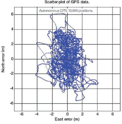
If the distribution really were circular then rms1 would the same in all directions, and so rms East would be the same as rms North. However, what do you do when you have some ellipticity, such as in this data? The answer is to work with rms2 as the entry point to the table. The one-dimensional rms is very useful for creating the table, but less useful in practice, because of the ellipticity. Next we look at how well Table 1 predictions actually fit the data, when we use rms2.

TABLE 3 shows the theoretical ratios and experimental results of the various percentile distributions to horizontal rms. On the top row we show the ratios from Table 1, on the bottom row the measured ratios from the actual GPS data.

Table 3. Theoretical ratios and experimental results using actual GPS data.

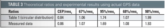
For our data: horizontal rms = rms2 = 2.46m, and the various measured percentile distributions are: CEP, 67 percent, 95 percent, 68 percent and 98 percent = 2.11, 2.62, 4.15, 2.65, and 4.74m respectively.

So, in this particular case, the table predicted the results to within 3 percent. With larger ellipticity you can expect the table to give worse results. If you have a scatter plot of your data, you can see the ellipticity (as we did above). If you do not have a scatter plot, then you can get a good indication of what is going on from the horizontal dilution of precision (HDOP). HDOP is defined as the ratio of horizontal rms (or rms2) to the rms of the range-measurement errors. If HDOP doubles, your position accuracy will get twice as bad, and so on. Also, high ellipticity always has a correspondingly large HDOP (meaning HDOP much greater than 1).

Galileo and Friends

Luckily for us, the future promises more satellites than the past. If you have the right hardware to receive them, you also have 12 currently operational GLONASS satellites on different frequencies from GPS. Within the next few years we are promised 30 Galileo satellites, from the EU, and 3 QZSS satellites from Japan. All of these will transmit on the same L1 frequency as GPS. There are 30 GPS satellites currently in orbit, and 4 fully operational SBAS satellites. Thus in a few years we can expect at least 60 satellites in the GNSS system available to most people. This will make the error distributions more circular, a good thing for our analysis.

Working with Actual Data

When it comes to data sets, we’ve seen that size certainly matters — with the simple case of dice as well as the more complicated case of GPS. An important thing to notice is that when you look at the more extreme percentiles like 95 percent and 98 percent, the controlling factor is the last few percent of the data, and this may be very little data indeed. Consider an example of 100 GPS fixes. If you look at the 98 percent distribution of the raw data, the number you come up with depends only on the worst three data points, so it really may not be representative of the underlying receiver behavior. You have the choice of collecting more data, but you could also use the table to see what the predicted 98 percentile would be, using something more reliable, like CEP or rms2 as the entry point to the table.

Conclusion

The “take-home” part of this article is Table 1, which you can use to convert one accuracy measure to another. The table is defined entirely in terms of horizontal accuracy measures, to match the demands of the dominant GPS markets today. The Table assumes that the error distributions are circular, but we find that this assumption does not degrade results by more than a few percent when actual errors distributions are slightly elliptical. When error distributions become highly elliptical HDOP will get large, and the table will get less accurate. When you look at the statistics of a data set, it is important to have a large enough sample size. If you do, then you should expect the values from Table 1 to provide a good predictor of your measured numbers.

Manufacturers

GPS receiver used for data collection: Global Locate (www.globallocate.com) Hammerhead single-chip host-based GPS.

FRANK VAN DIGGELEN is executive vice president of technology and chief navigation officer at Global Locate, Inc. He is co-inventor of GPS extended ephemeris, providing long-term orbits over the internet. For this and other GPS inventions he holds more than 30 US patents. He has a Ph.D. E.E. from Cambridge University.