Converging on the jammer: Dual-satellite GPS interference localization from space

No audio available for this content.

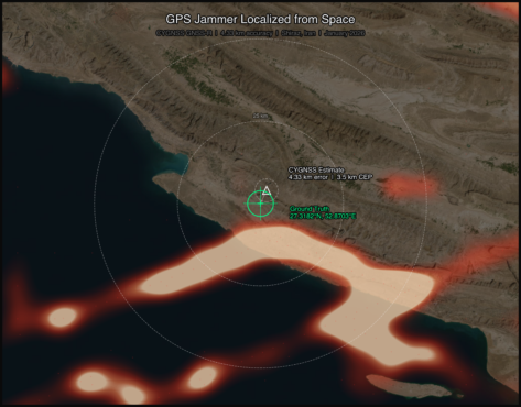
On a January morning in 2026, a GPS jammer powered up near Shiraz, Iran. It was not the first, and it would not be the last. The Strait of Hormuz corridor has become one of the most persistently jammed airspaces on Earth. But this time, two satellites were watching from very different vantage points, and together they would demonstrate something new: that spaceborne sensors can localize a terrestrial GPS jammer to within a few kilometers, using physics alone.

This article presents the first direct comparison of Cyclone Global Navigation Satellite System (CYGNSS) — a NASA GNSS reflectometry constellation — and NASA-ISRO Synthetic Aperture Radar (NISAR) — an L-band synthetic aperture radar for GPS jammer localization. The results challenge assumptions about which modality performs better and reveal that the answer depends on a question most analysts forget to ask.

The setup: Known jammer, known position

Validation requires ground truth. With help from the PNT community, we identified a GPS jammer operating near 27.32°N, 52.87°E (approximately 50 km southwest of Shiraz) that was active on Jan. 8 and Jan. 20, 2026, with confirmed quiet periods on Dec. 15 and Dec. 27, 2025. The jammer’s position was established through independent signals intelligence.

This gave us a controlled experiment: two “jammer ON” dates and two “jammer OFF” baseline dates, with satellite coverage from both CYGNSS and NISAR spanning the full period.

Two satellites, two physics

CYGNSS is a constellation of eight microsatellites that measure GPS signals reflected off Earth’s surface. Each spacecraft carries a delay-Doppler receiver that maps reflected signal power across a grid of delay and Doppler bins, known as the delay-Doppler map, or DDM. When a terrestrial jammer is active, it floods the GPS band with noise, elevating the DDM noise floor and suppressing the coherent surface reflection. The effect is detectable hundreds of kilometers from the jammer, creating a wide-area footprint in the reflected signal data.

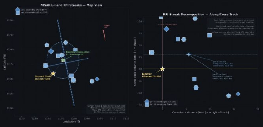
NISAR operates an L-band SAR at 1.257 GHz, just 30 MHz from the GPS L2 frequency at 1.2276 GHz. When a GPS jammer’s broadband emissions leak into NISAR’s receive band, they create characteristic streaks in the SAR imagery. The streaks are elongated in the cross-track (range) direction, not along-track, a counterintuitive result that follows directly from SAR signal processing. In azimuth (along-track), the jammer is a fixed-point source with a valid Doppler history, so the SAR azimuth processor focuses it correctly, similar to any ground target. But in range (cross-track), the jammer’s broadband noise does not match the SAR’s chirp waveform, so range compression smears the energy across many range bins rather than compressing to a point. The result is a streak perpendicular to the flight direction, whose along-track centroid encodes the jammer’s latitude and whose cross-track extent encodes a range arc, which is the distance from the orbit ground track (FIGURE 1). The bearing of each streak encodes the jammer’s direction relative to the satellite’s ground track.

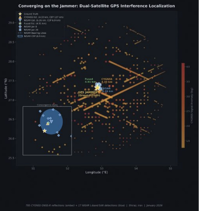
The two sensors could hardly be more different. CYGNSS sees the jammer’s effect on reflected GPS signals, offering an indirect measurement spread across hundreds of specular reflection points. NISAR sees the jammer’s emissions directly in its own receiver, which is a more precise measurement, but only along the satellite’s narrow ground track. FIGURE 2 shows both detection sets converging on the jammer location.

CYGNSS: 785 Detections, 4.33 km Error

We processed all CYGNSS Level 1 data within 200 km of the jammer location on both ON and OFF dates. Four detection methods contributed observations:

■ DDM noise floor (419 detections): The pre-computed ddm_noise_floor variable, calibrated against the thermal noise reference, proved the strongest discriminator. Near-jammer values exceeded 15,000 counts against a ~10,000 mean background.

■ Spatial noise grid (299):A 10 km gridded analysis identified cells with anomalously elevated noise relative to adjacent cells.

■ SNR hole detection (66): Coherent surface reflections were suppressed near the jammer, creating spatial “holes” in the SNR field.

■ NBRCS drop (1): Surface reflectivity dropped approximately 16% near the jammer, though this method produced few threshold exceedances.

Across four DDM channels per spacecraft and multiple passes, this yielded 785 total anomalous observations on the jammer-ON dates.

Localizing using a simple centroid of all 785 detection positions placed the jammer 32.1 km from truth, with too many distant, low-SNR detections diluting the estimate.

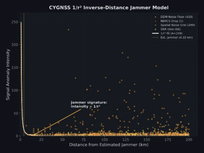
Instead, we fit a parametric 1/r² inverse-distance model:

I(r)=Ar2

where A is a free amplitude parameter and r is the distance from a candidate jammer position. We jointly optimized the jammer position and amplitude using SciPy’s Nelder-Mead optimizer across all 785 observations, weighted by intensity. The optimizer converged on a position 4.33 km from ground truth, providing a 27.7 km improvement over the centroid (FIGURE 3).

The baseline: Zero false positives

On the jammer-OFF dates (Dec. 15 and Dec. 27, 2025), the pipeline produced exactly zero detections using the same thresholds, geographic area and satellites: a completely clean result. This suggests that the 785 detections are unlikely to be sensor artifacts or geographic anomalies. They disappear when the jammer turns off.

NISAR: 17 Detections, 6.26 km Error

NISAR’s approach is fundamentally different. Rather than measuring hundreds of reflected signals across a wide area, it captures direct emissions in a narrow swath, but with far greater geometric precision.

We processed NISAR L2 GCOV (geocoded covariance) products from Track 157, Frame 15 (ascending) for three dates: the Dec. 27 baseline and the Jan. 8 and Jan. 20 jammer-ON passes. The detection pipeline used eigenvalue decomposition of the polarimetric covariance matrix:

1. λ₁ ratio thresholding: In jammer-contaminated pixels, the dominant eigenvalue λ₁ of the 2×2 [HH, HV] covariance matrix rises sharply relative to the scene mean, indicating an unpolarized additive source.
2. Cross-polarization ratio (HV/HH): GPS jammer emissions are unpolarized, disproportionately elevating the HV channel. Anomalous HV/HH ratios flag contaminated azimuth lines.
3. Iterative outlier trimming: Three rounds of 1.5σ clipping removed scattered false detections, leaving 17 high-confidence streak centroids.

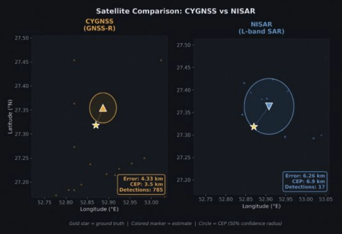
With detections from two passes on different dates, we had two independent bearing lines. Each pass’s streak centroids defined an azimuth aligned cluster whose major axis pointed toward the jammer. A PCA fit to the two clusters extracted the bearing: 308.1° from the Jan. 8 pass and 316.2° from Jan. 20. Their intersection — computed via scipy optimization of the angular residual — landed 6.26 km from ground truth (FIGURE 4).

The along-track/cross-track decomposition reveals why the 6.26 km error is a geometric ceiling for this dataset, not a processing limitation. Both passes come from the same Track 157 ascending orbit on a 12-day repeat cycle. The intensity-weighted along-track centroids land at +3.0 km and +3.1 km north of the jammer, a direct stable latitude measurement. The cross-track centroids land at +5.4 km and +5.6 km east of the orbit ground track, a range measurement. But because both passes share identical orbit geometry, the two range arcs are nearly parallel. The bearing difference between passes (308.1° vs 316.2°) is only 8.1°, producing a shallow intersection angle and poor cross-range resolution. A single descending pass, which would cross the ascending track at approximately 60-70°, would transform the geometry from two near-parallel lines to a genuine triangulation, potentially reducing the localization error to sub-2 km. Unfortunately, no descending NISAR pass covering this jammer site was available in the beta archive, which ends on Jan. 20, 2026.

The CEP (circular error probable, the radius containing 50% of repeated estimates) was 6.88 km, meaning if we ran this analysis on many similar jammers, half our estimates would fall within ~7 km.

Who wins?

CYGNSS wins, and not just on accuracy.

A naive confidence metric for the 1/r² fit would be the scatter of the 785 input detections (CEP = 127 km). But the detections are not the estimate; they are the inputs to a model fit. The relevant confidence question is: How stable is the fitted position?

We answered this with a 500-iteration bootstrap: resample the 785 detections with replacement, re-run the 1/r² optimizer each time and measure the spread of the resulting position estimates. The bootstrap CEP, the median radial distance across 500 fitted positions, was 3.48 km. The optimizer converges stably to within a few kilometers of the same location regardless of which detections are included.

This means CYGNSS achieves 4.33 km error with 3.48 km confidence, both better than NISAR’s 6.26 km error and 6.88 km confidence.

The bootstrap CEP also reveals what the raw scatter obscures: the 1/r² fit is constrained primarily by the ~80 high-intensity detections within 30 km of the jammer. The remaining 700 distant, low-intensity detections contribute little to the position estimate — they are correctly downweighted by the intensity-weighted least squares. The fit’s stability comes from the physics: a 1/r² signal has steep gradients near the source, providing strong positional constraints where it matters most.

Bayesian fusion: Can we get both?

The obvious next question: Can we combine CYGNSS’s wide-area sensitivity with NISAR’s geometric precision? We implemented four fusion strategies, all designed to work without ground truth:

■ Bayesian Gaussian posterior: Model each sensor’s estimate as a 2D isotropic Gaussian with σ = CEP/1.1774. The posterior is the product of the two Gaussians: an analytical precision-weighted mean.

■ NISAR-prior constrained 1/r²: Re-run the CYGNSS optimizer with a Gaussian regularization term pulling toward the NISAR estimate, sweeping the regularization weight λ from 0.01 to 10.

■ NISAR-proximity re-weighted 1/r²: Apply a Gaussian kernel centered on the NISAR estimate to the CYGNSS detections before fitting, effectively upweighting observations consistent with the SAR result.

■ Joint CEP-balanced: Combine the CYGNSS gradient signal with NISAR cluster proximity, weighted by (σ_CYGNSS/σ_NISAR)².

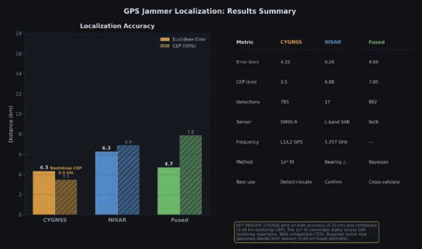
With the bootstrap CEP, the precision ratio flips. The CYGNSS Gaussian (σ = 2.95 km) is now 2× tighter than NISAR (σ = 5.84 km). The Bayesian posterior, the precision-weighted mean, lands at 4.69 km, pulling toward CYGNSS’s better estimate while incorporating NISAR’s independent geometric constraint. FIGURE 5 shows the fusion: two comparable Gaussians whose product is tighter than either alone.

The fused result (4.69 km error, 7.85 km CEP) is not quite as accurate as CYGNSS alone (4.33 km), because NISAR’s 6.26 km estimate pulls it slightly away from truth. But operationally, the fusion provides a cross-validated answer: two independent physics arriving at similar locations builds confidence that neither sensor is producing an artifact.

The key insight is that the bootstrap CEP unlocked meaningful fusion. When the raw scatter CEP (127 km) was used, NISAR dominated the posterior 343:1 and fusion added nothing. With the fit-based CEP (3.48 km), both sensors contribute, and the posterior reflects genuine multi-modal evidence.

Operational implications

For CYGNSS: CYGNSS excels at both detection and localization. Its 785 detections across a 200 km radius, with zero false positives on baseline dates, provide unambiguous jammer detection. The 1/r² fit achieves 4.33 km accuracy with a bootstrap-verified 3.48 km CEP, meaning an analyst can trust the result to single-digit kilometer precision without ground truth. CYGNSS’s eight-satellite constellation also provides sub-daily revisit, enabling near-real-time monitoring.

For NISAR: NISAR provides independent geometric confirmation. With just two passes over an active jammer, the bearing intersection achieved 6.26 km accuracy with a 6.88 km CEP. The 6.26 km result is constrained by orbit geometry, not by detection sensitivity. Our two ascending passes from Track 157 produced nearly parallel range arcs with only 8.1° of bearing separation. Adding a single descending pass would provide a crossing angle of 60° to 70° and could reduce localization error to sub-2 km — transforming NISAR from a confirming sensor into a precision localization tool in its own right. The limitation in this study was data availability: The NISAR beta archive contained only ascending Track 157 passes over the jammer site. NISAR’s 12-day repeat cycle and fixed ground track also mean the jammer must be active when the satellite passes overhead. NISAR’s current value is as a confirming sensor — when both modalities converge on the same location, confidence increases beyond what either achieves alone.

For Fusion: With comparable CEPs (3.48 km vs 6.88 km), fusion now produces genuinely blended estimates. The Bayesian posterior at 4.69 km reflects real multi-sensor information. Future improvements, such as more NISAR passes with diverse bearings or CYGNSS multi-week accumulation, would tighten both estimates further.

For the Adversary: These results demonstrate that GPS jammers operating in contested airspace are observable and localizable from orbit using openly available civilian satellite data. The 4.33 km CYGNSS result is approximately 2× better than the published state of the art for GNSS-R jammer localization (~9 km grid resolution, Chew et al., 2023) and the NISAR bearing intersection approach has not been previously demonstrated for jammer geolocation.

Still broadcasting: Jammer persistence through conflict

The validation analysis used January 2026 data. But on Feb. 28, armed conflict erupted in the region. Did the jammer survive?

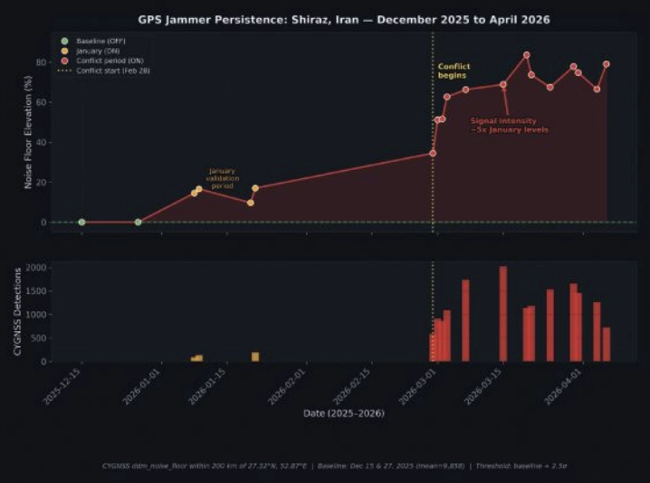
We ran the CYGNSS noise floor detection pipeline for each day from Feb. 28 through April 6, comparing against the December 2025 baseline. The answer is unambiguous: The jammer is not only still active — it is operating at dramatically higher power.

In January, the jammer elevated the CYGNSS noise floor by approximately 15% above baseline. By early March, days after the conflict began, noise elevation had jumped to 50% to 60%. By mid-March, it reached 70% to 84%, where it remained through early April. Detection counts tell the same story: 89 to 192 per day in January, rising to 1,000 to 2,000 per day during the conflict (FIGURE 6).

The escalation was immediate. On Feb. 28, noise elevation was +34.5%, already double the January level. By March 3, it had reached +62.7%, and by April 6, it peaked at +79.1%. The signal has remained at 5× the January intensity through the most recent available data (April 6, 2026).

Several interpretations are consistent with this pattern:

■ Power increase: The operator increased jammer output power, perhaps in response to the conflict or as a defensive posture against GPS-guided munitions.

■ Additional jammers: Multiple units may have been co-located or deployed nearby, creating an aggregate signature larger than any single device.

■ Duty cycle change: The jammer may have shifted from intermittent to continuous operation.

What is clear is that the jammer we localized in January was not incapacitated by the conflict. It was amplified. CYGNSS’s sub-daily revisit capability makes this kind of persistent monitoring possible using entirely passive, civilian satellite data — no tasking, no cooperation with the target state and no risk to reconnaissance assets.

Context and prior work

CYGNSS-based RFI detection builds on work by Chew et al., 2023, who demonstrated grid-level jammer detection at approximately 9 km resolution using DDM noise floor anomalies. Our 1/r² parametric fit extends this from detection to localization, achieving sub-5 km accuracy by exploiting the physics of signal power decay.

At the other end of the precision spectrum, Murrian et al., 2021, demonstrated ~220 m jammer localization using ISS-mounted Doppler measurements of raw intermediate-frequency (IF) data. This approach achieves an order of magnitude better precision than our methods but requires specialized hardware and raw signal access not available on current operational satellites.

The NISAR bearing intersection approach demonstrated here is, to our knowledge, the first published use of L-band SAR RFI streaks for jammer triangulation. The key insight is that NISAR’s proximity to GPS L2 (just 30 MHz separation) makes it an unintentional but effective GPS interference sensor.

Summary

Two satellites, two physics, one jammer. CYGNSS sees the interference footprint across hundreds of kilometers and localizes the source through inverse-distance physics. NISAR sees the emissions directly in its SAR receiver and triangulates through bearing intersection. Both achieve sub-7 km accuracy independently; together, they cross-validate and build the confidence that operational use demands.

The jammer near Shiraz is still there — louder than ever. The satellites are still watching.